Ed Nisley's Blog: Shop notes, electronics, firmware, machinery, 3D printing, laser cuttery, and curiosities. Contents: 100% human thinking, 0% AI slop.
Category: Science
If you measure something often enough, it becomes science
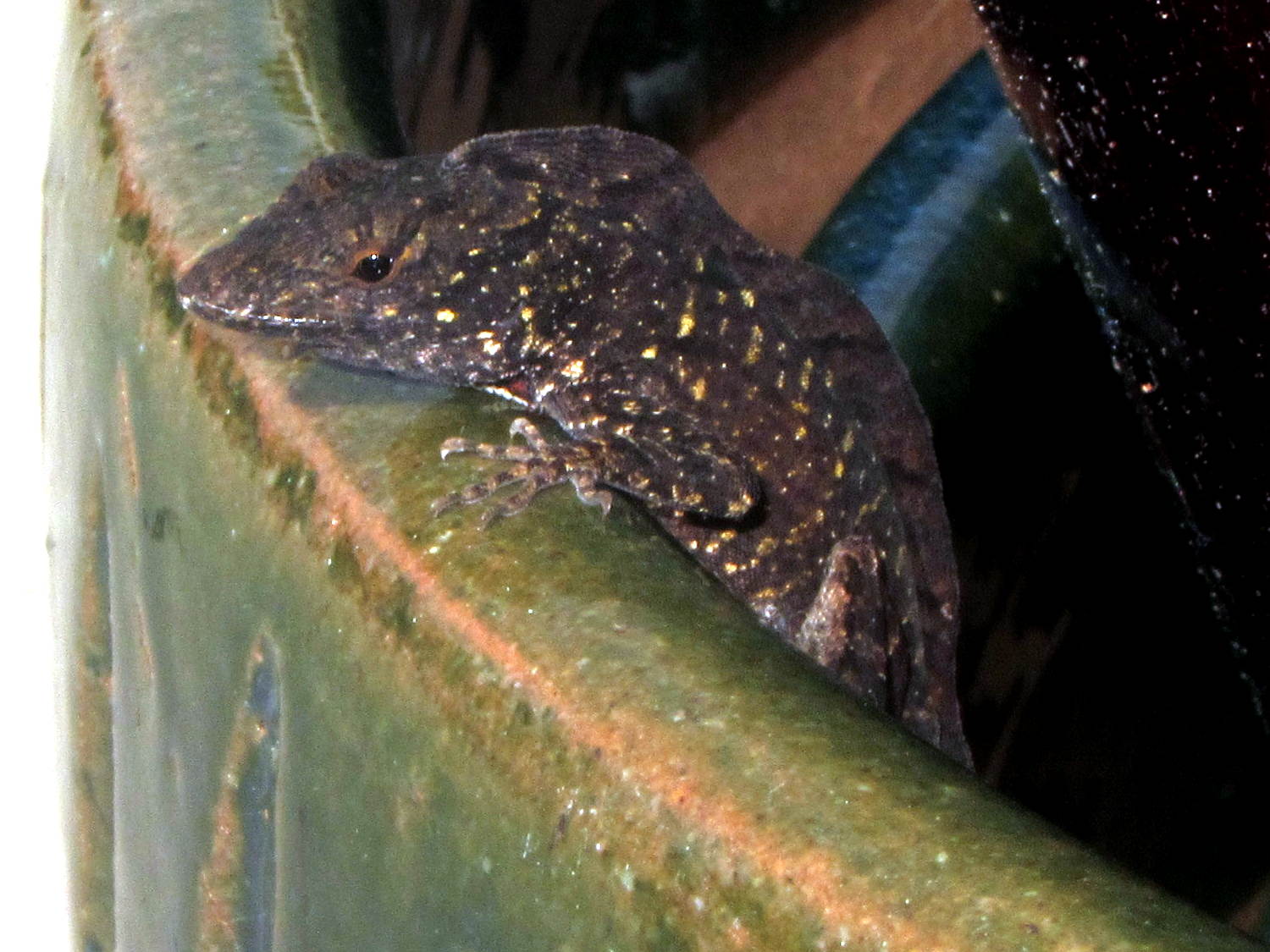
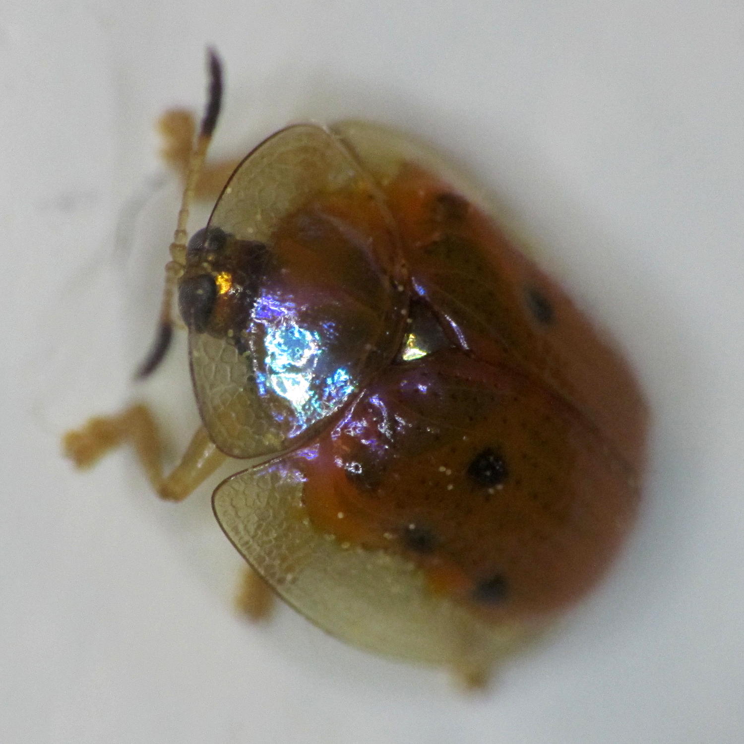
We found this critter keeping a watchful eye on the construction at Adams Fairacre Farms during our most recent grocery trip:
Mystery frilled lizard – detail
I think it’s an undocumented alien that entered the US stowed away in a tropical plant, because it was affixed to the array of ceramic pots outside their (open) greenhouse windows:
Mystery frilled lizard
To the best of my admittedly limited herpetological knowledge, none of our native lizards / geckos / whatever have such a distinctive dorsal frill / fin / ridge. I have no idea how to look the critter up, though.
We left it to seek its own destiny. Unless it’s a mated female (hard to tell with lizards), it’ll have a lonely life.
Perhaps it practices rishratha, which is entirely possible.
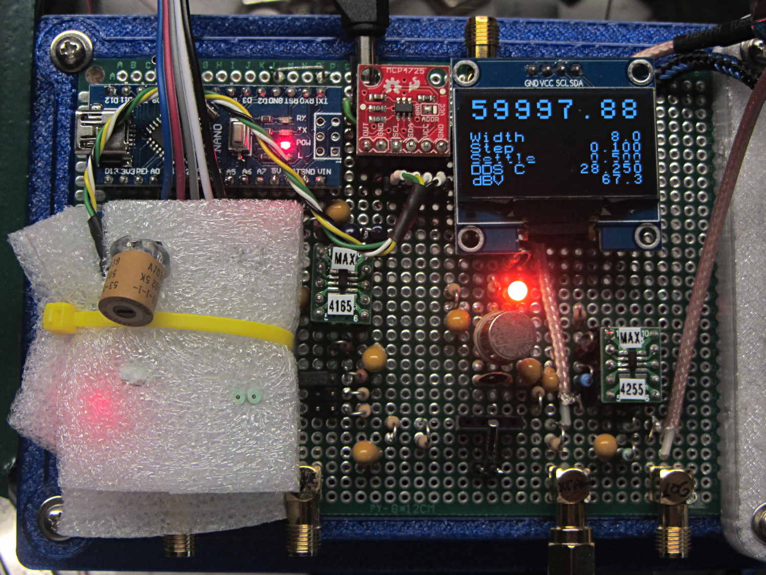
With an LM75 atop the 125 MHz oscillator and the whole thing wrapped in foam:
LM75A Temperature Sensor – installed
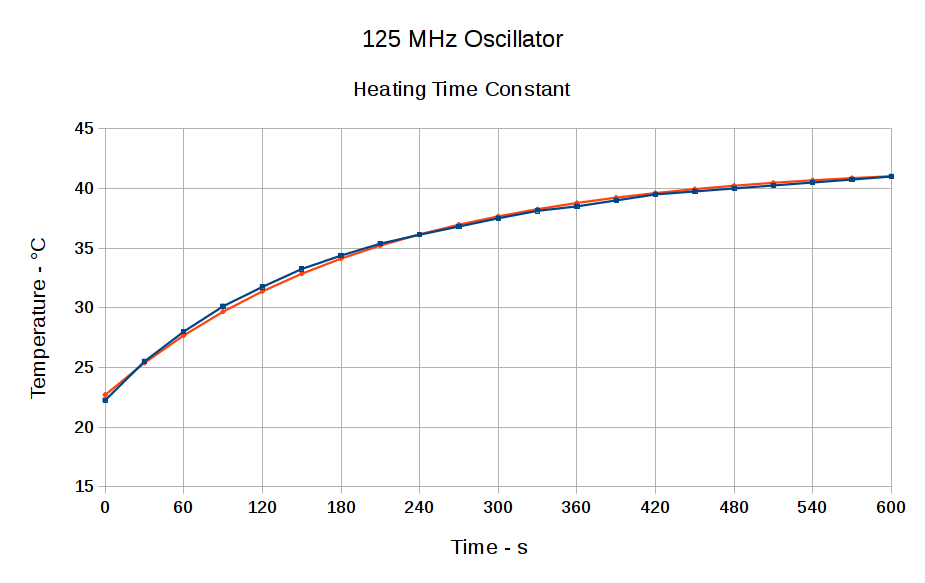
Let it cool overnight in the Basement Laboratory, fire it up, record the temperature every 30 seconds, and get the slightly chunky blue curve:
125 MHz Oscillator – Heating Time Constant
Because we know this is one of those exponential-approach problems, the equation looks like:
Temp(t) = Tfinal + (Tinit - Tfinal) × e-t/τ
We can find the time constant by either going through the hassle of an RMS curve fit or just winging it by assuming:
The initial temperature, which is 22.5 °C = close to 22.7 °C ambient
The final temperature (call it 42 °C)
Any good data point will suffice
The point at 480 s is a nice, round 40 °C, so plug ’em in:
40.0 = 42.0 + (22.7 - 42.0) × e-480/τ
Turning the crank produces τ = 212 s, which looks about right.
Trying it again with the36.125 °C point at 240 s pops out 200.0 °C.
Time for a third opinion!
Because we live in the future, the ever-so-smooth red curve comes from unleashing LibreOffice Calc’s Goal Seek to find a time constant that minimizes the RMS Error. After a moment, it suggests 199.4 s, which I’ll accept as definitive.
The spreadsheet looks like this:
T_init
22.5
T_final
42.0
Tau
199.4
Time s
Temp °C
Exp App
Error²
0
22.250
22.500
0.063
30
25.500
25.224
0.076
60
28.000
27.567
0.187
90
30.125
29.583
0.294
120
31.750
31.317
0.187
150
33.250
32.810
0.194
180
34.375
34.093
0.079
210
35.375
35.198
0.031
240
36.125
36.148
0.001
270
36.813
36.965
0.023
300
37.500
37.668
0.028
330
38.125
38.273
0.022
360
38.500
38.794
0.086
390
39.000
39.242
0.058
420
39.500
39.627
0.016
450
39.750
39.959
0.043
480
40.000
40.244
0.059
510
40.250
40.489
0.057
540
40.500
40.700
0.040
570
40.750
40.882
0.017
600
41.000
41.038
0.001
RMS Error
0.273
The Exp App column is the exponential equation, assuming the three variables at the top, the Error² column is the squared error between the measurement and the equation, and the RMS Error cell contains the square root of the average of those squared errors.
The Goal Seeker couldn’t push RMS Error to zero and gave up with Tau = 199.4. That’s sensitive to the initial and final temperatures, but close enough to my back of the envelope to remind me not to screw around with extensive calculations when “two minutes” will suffice.
Basically, after five time constants = 1000 s = 15 minutes, the oscillator is stable enough to not worry about.
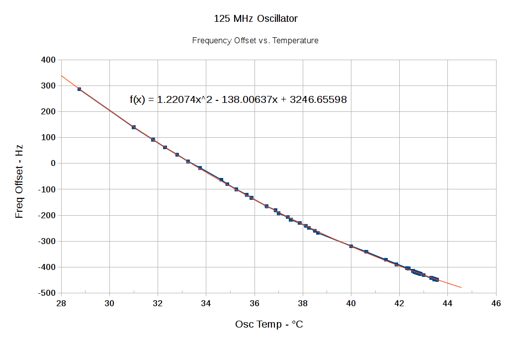
I let the DDS cool down overnight, turned it on, and recorded the frequency offset as a function of temperature as it heated up again:
125 MHz Osc Freq Offset vs Temp – Quadratic – 29 – 43 C
The reduced spacing between the points as the temperature increases shows how fast the oscillator heats up. I zero-beat the 10 MHz output, scribbled the temperature, noted the offset, and iterated as fast as I could. The clump of data over on the right end comes from the previous session with essentially stable temperatures.
I only had to throw out two data points to get such a beautiful fit; the gaps should be obvious.
The fit seems fine from room (well, basement) ambient up to hotter than you’d really like to treat the DDS, so using the quadratic equation should allow on-the-fly temperature compensation. Assuming, of course, the equation matches some version of reality close to the one prevailing in the Basement Laboratory, which remains to be seen.
In truth, it probably doesn’t, because the temperature was changing so rapidly the observations all run a bit behind reality. You’d want a temperature-controlled environment around the PCB to let the oscillator stabilize after each increment, then take the measurements. I am so not going to go there.
The original data:
125 MHz Osc Freq Offset vs Temp – 29 – 43 C – data
DDS Oscillator Frequency Offset vs. Temperature – complete
Now, as it turns out, the one lonely little dot off the line happened just after I lit the board up after a tweak, so the oscillator temperature hadn’t stabilized. Tossing it out produces a much nicer fit:
DDS Oscillator Frequency Offset vs. Temperature
Looks like I made it up, doesn’t it?
The first-order coefficient shows the frequency varies by -36 Hz/°C. The actual oscillator frequency decreases with increasing temperature, which means the compensating offset must become more negative to make the oscillator frequency variable match reality. In previous iterations, I’ve gotten this wrong.
For example, at 42.5 °C the oscillator runs at:
125.000000 MHz - 412 Hz = 124.999588 MHz
Dividing that into 232 = 34.35985169 count/Hz, which is the coefficient converting a desired frequency into the DDS delta phase register value. Then, to get 10.000000 MHz at the DDS output, you multiply: 10×106 × 34.35985169 = 343.598517×10⁶
Stuff that into the DDS and away it goes.
Warmed half a degree to 43.0 °C, the oscillator runs at:
125.000000 MHz - 430 Hz = 124.999570 MHz
That’s 18 Hz lower, so the coefficient becomes 34.35985667, and the corresponding delta phase for a 10 MHz output is 343.598567×10⁶.
After insulating the DDS module to reduce the effect of passing breezes, I thought the oscillator temperature would track the ambient temperature fairly closely, because of the more-or-less constant power dissipation inside the foam blanket. Which turned out to be the case:
DDS Oscillator Temperature vs. Ambient
The little dingle-dangle shows startup conditions, where the oscillator warms up at a constant room temperature. The outlier dot sits 0.125 °C to the right of the lowest pair of points, being really conspicuous, which was another hint it didn’t belong with the rest of the contestants.
So, given the ambient temperature, the oscillator temperature will stabilize at 0.97 × ambient + 20.24, which is close enough to a nice, even 20 °C hotter.
The insulation blanket reduces short-term variations due to breezes, which, given the -36 Hz/°C = 0.29 ppm temperature coefficient, makes good sense; you can watch the DDS output frequency blow in the breeze. It does, however, increase the oscillator temperature enough to drop the frequency by 720 Hz, so you probably shouldn’t use the DDS oscillator without compensating for at least its zero-th order offset at whatever temperature you expect.
Of course, that’s over a teeny-tiny temperature range, where nearly anything would be linear.
The two knockoff Neopixeltestfixtures went dark while their USB charger accompanied me on a trip, so they spent a few days at ambient basement conditions. When I plugged them back into the charger, pretty much the entire array lit up in pinball panic mode:
WS2812 LED – test fixture multiple failures
Turns out three more WS2812 chips failed in quick succession. I’ve hotwired around the deaders (output disconnected, next chip input in parallel) and, as with the other zombies, they sometimes work and sometimes flicker. That’s five failures in 28 LEDs over four months, a bit under 3000 operating hours.
For lack of a better explanation: the cool chips pulled relatively moist air through their failed silicone encapsulation, quietly rotted out in the dark, then failed when reheated. After they spend enough time flailing around, the more-or-less normal operating temperatures drives out the moisture and they (sometimes) resume working.
Remember, all of them passed the Josh Sharpie Test, so you can’t identify weak ones ahead of time.
A slight modification spits out the (actual) frequency and dBV response (without subtracting the 108 dB intercept to avoid negative numbers for now) to the serial port in CSV format, wherein a quick copypasta into a LibreOffice Calc spreadsheet produces this:
Spectrum-32
Changing the center frequency and swapping in a 60 kHz resonator:
Spectrum-60
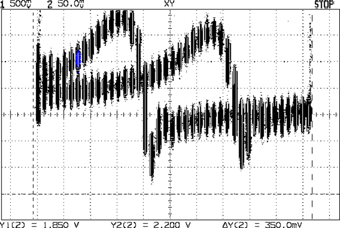
Much prettier than the raw scope shot with the same data, there can be no denyin’:
Log V vs F – 32766 4 Hz – CX overlay
I think the wobbulations around the parallel resonant dip come from the excessively hugely too large 10 µF caps in the signal path, particularly right before the log amp input, although the video bandwidth hack on the AD8310 module may contribute to the problem. In any event, I can see the log amp output wobbling for about a second, which is way too long.
Anyhow, the series-resonant peaks look about 1 Hz wide at the -3 dBV points, more or less agreeing with what I found with the HP 8591 spectrum analyzer. The series cap is a bit smaller, producing a slightly larger frequency change in the series resonant frequency: a bit under 2 Hz, rather than the 1 Hz estimated with the function generator and spectrum analyzer.
I still don’t understand why the parallel resonant dip changes, although I haven’t actually done the pencil pushing required for true understanding.