Ed Nisley's Blog: Shop notes, electronics, firmware, machinery, 3D printing, laser cuttery, and curiosities. Contents: 100% human thinking, 0% AI slop.
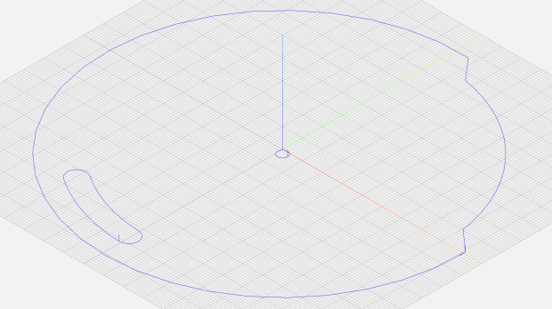
Two passes make the scratch deep enough to hold engraving crayon / lacquer / ink, without making it much wider. Laser engraving would surely work better.
In lieu of actually milling the cursor, this code scratches the perimeter:
local dr = DeckBottomOD/2;
local hr = CursorHubOD/2;
local a = atan(hr - CursorTipWidth/2,dr); // rough & ready approximation
local p0 = hr * [sin(a),cos(a),-]; // upper tangent point on hub
local c1 = [dr - CursorTipRadius,CursorTipWidth/2 - CursorTipRadius*cos(a),-];
local p1 = c1 + [CursorTipRadius*sin(a),CursorTipRadius*cos(a),-];
local p2 = c1 + [CursorTipRadius,0,-]; // around tip radius
feedrate(KnifeSpeed);
goto([-,-,TravelZ]);
goto([-hr,0,-]);
move([-,-,EngraveZ]);
repeat(3) {
arc_cw(p0,hr);
move(p1);
arc_cw(p2,CursorTipRadius);
move([p2.x,-p2.y,-]);
arc_cw([p1.x,-p1.y,-],CursorTipRadius);
move([p0.x,-p0.y,-]);
arc_cw([-hr,0,-],hr);
}
Three passes makes it deep enough to snap along the line:
Tektronix Circuit Computer – cursor outline
If you look closely, though, you’ll find a little divot over on the left along the bottom edge, so I really must machine the thing.
Were I to go into production, I’d have to figure out a fixture, but I think I can just clamp a rough-cut acrylic rectangle to the Sherline’s table, mill half the perimeter, re-clamp without moving anything, then mill the other half.
Subtractive machining is such a bother!
The pivot holding the cursor and decks together is a “Chicago screw“, a.k.a. a “sex bolt“. I am not making this up.
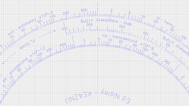
The Tektronix Circuit Computer, being a specialized circular slide rule, requires logarithmic scales bent around arcs:
Scale Tick Layout – Bottom Deck
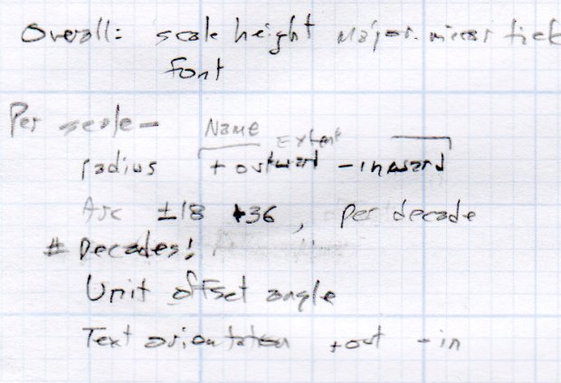
Each decade spans 18°, except for the FL scale’s 36° span to extract the square root of the LC product:
FL = 1 / (2π · sqrt(LC))
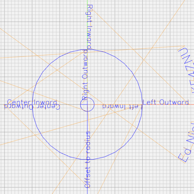
The tick marks can point inward or outward from their baseline radius, with corresponding scale labels reading either inward or outward.
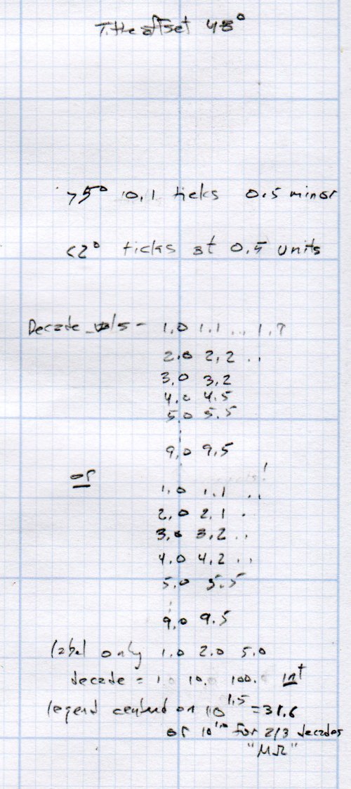
There being no (easy) way to algorithmically set the tick lengths, I used a (pair of) tables (a.k.a. vector lists):
TickScaleNarrow = {
[1.0,TickMajor],
[1.1,TickMinor],[1.2,TickMinor],[1.3,TickMinor],[1.4,TickMinor],
[1.5,TickMid],
[1.6,TickMinor],[1.7,TickMinor],[1.8,TickMinor],[1.9,TickMinor],
[2.0,TickMajor],
[2.2,TickMinor],[2.4,TickMinor],[2.6,TickMinor],[2.8,TickMinor],
[3.0,TickMajor],
… and so on …
The first number in each vector is the tick value in the decade, the log of which corresponds to its angular position. The second gives its length, with three constants matching up to the actual lengths on the Tek scales.
The Circuit Computer labels only three ticks within each decade in the familiar (to EE bears, anyhow) 1, 2, 5 sequence. Their logs are 0.0, 0.3, and 0.7, spacing them neatly at the 1/3 decade points.
Pop quiz: If you wanted to label two evenly spaced ticks per decade, you’d mark 1 and …
Generating the L (inductance) scale on the bottom deck goes like this:
The L scale covers 1 nH to 1 MH (!), as set by the MinLog and MaxLog values. Arc sets the angular size of each decade from ScaleArc, with the negative sign indicating the values increase in the clockwise direction.
The first decade starts with a tick labeled 1, so dec = 1. The next decade has dec = 10 and the third has dec = 100. Maybe I should have used the log values 0, 1, and 2, but that seemed too intricate.
The angular offset is zero because this is the outermost scale, so 1.0 H will be at 0° (the picture is rotated about half a turns, so you’ll find it off to the left). All other scales on the deck have a nonzero offset to put their unit tick at the proper angle with respect to this one.
The scales have legends for each group of three decades, positioned in the middle of the group:
I wish there were a clean way to draw exponents, as the GCMC Hershey font does not include superscripts, but the characters already live at the small end of what’s do-able with a ballpoint pen cartridge. Engraving will surely work better, but stylin’ exponents are definitely in the nature of fine tuning.
With all that in hand, the scales look just like they should:
This file contains hidden or bidirectional Unicode text that may be interpreted or compiled differently than what appears below. To review, open the file in an editor that reveals hidden Unicode characters.
Learn more about bidirectional Unicode characters
This file contains hidden or bidirectional Unicode text that may be interpreted or compiled differently than what appears below. To review, open the file in an editor that reveals hidden Unicode characters.
Learn more about bidirectional Unicode characters
This file contains hidden or bidirectional Unicode text that may be interpreted or compiled differently than what appears below. To review, open the file in an editor that reveals hidden Unicode characters.
Learn more about bidirectional Unicode characters
The text baseline sits at the specified radius from the center point, regardless of its orientation, so you must offset the text path by half its height in the proper direction before handing it to the ArcText function.
A utility function to draw scale legends stuffs some of that complexity into a bottle:
function ArcLegend(Text,Radius,Angle,Orient) {
local tp = scale(typeset(Text,TextFont),LegendTextSize);
local tpa = ArcText(tp,[0mm,0mm],Radius,Angle,TEXT_CENTERED,Orient);
feedrate(TextSpeed);
engrave(tpa,TravelZ,EngraveZ);
}
Which means most of the text uses a simpler invocation:
Arc determines the angular span of each decade, with positive values going counterclockwise. MinLog is the logarithm of the scale endpoint, so adding 1.5 puts the text angle one-and-a-half decades from MinLog and multiplying by Arc moves it in the right direction. The offset angle rotates the entire scale with respect to the 0° reference sticking out the X axis over on the right. The top picture has its 0° reference pointing north-northeast.
The GCMC source code as a GitHub Gist:
This file contains hidden or bidirectional Unicode text that may be interpreted or compiled differently than what appears below. To review, open the file in an editor that reveals hidden Unicode characters.
Learn more about bidirectional Unicode characters
GCMC treats variables defined inside a function as local, unless they’re already defined in an enclosing scope, whereupon you overwrite the outer variables. This wasn’t a problem in my earlier programs, but I fired the footgun with nested functions using the same local / temporary variables. Now, I ruthlessly declare truly local variables as local, except when I don’t, for what seem good reasons at the time.
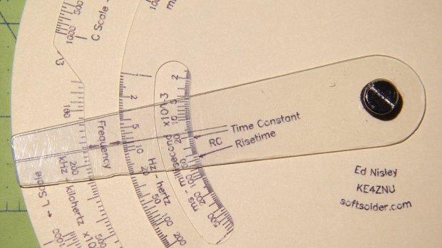
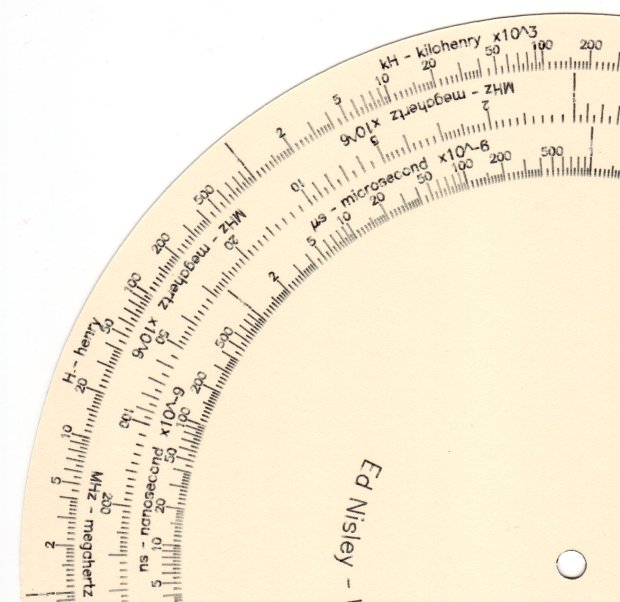
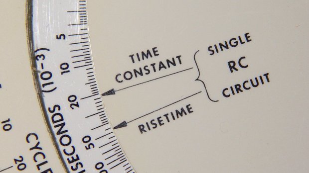
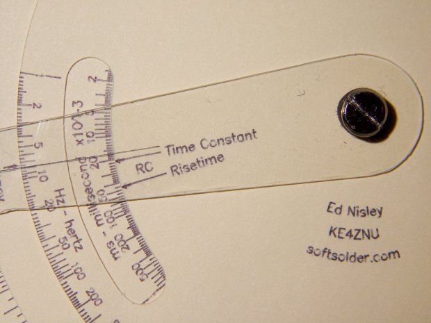
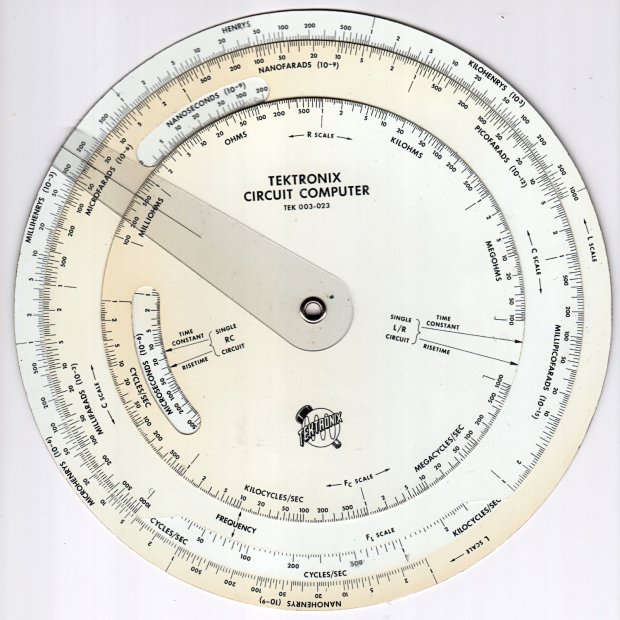
Following a linkie I can no longer find led me to retrieve the Tektronix Circuit Computer in my Box o’ Slide Rules:
Tektronix Circuit Computer – front
I’m pretty sure it came from Mad Phil’s collection. One can line up the discolored parts of the decks under their cutout windows to restore it to its previous alignment; most likely it sat at the end of a row of books (remember books?) on his reference shelf.
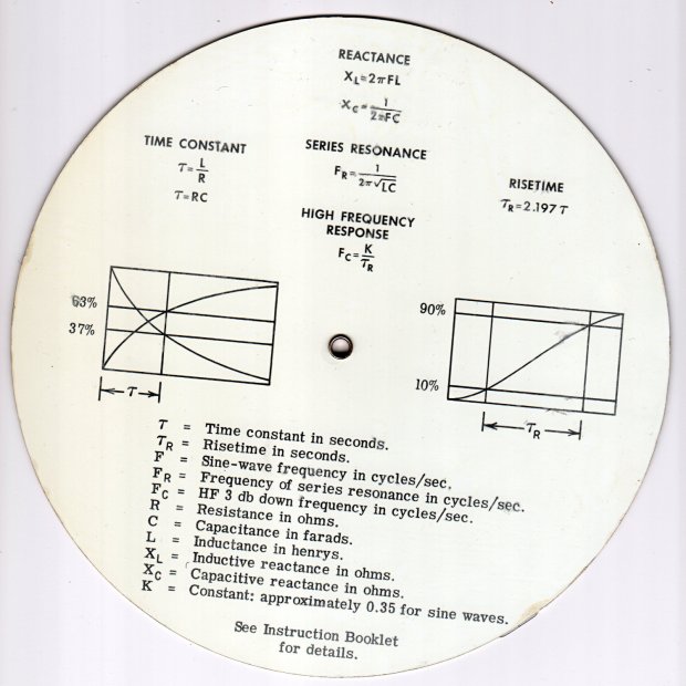
The reverse side lists the equations it can solve, plus pictorial help for the puzzled:
Tektronix Circuit Computer – rear
Some searching reveals the original version had three aluminum disks, shaped and milled and photo-printed, with a honkin’ hex nut holding the cursor in place. The one I have seems like laser-printed card stock between plastic laminating film; they don’t make ’em like that any more, either.
TEK PN 003-023 (the paper edition) runs about thirty bucks (modulo the occasional outlier) on eBay, so we’re not dealing in priceless antiquity here. The manual is readily available as a PDF, with photos in the back.
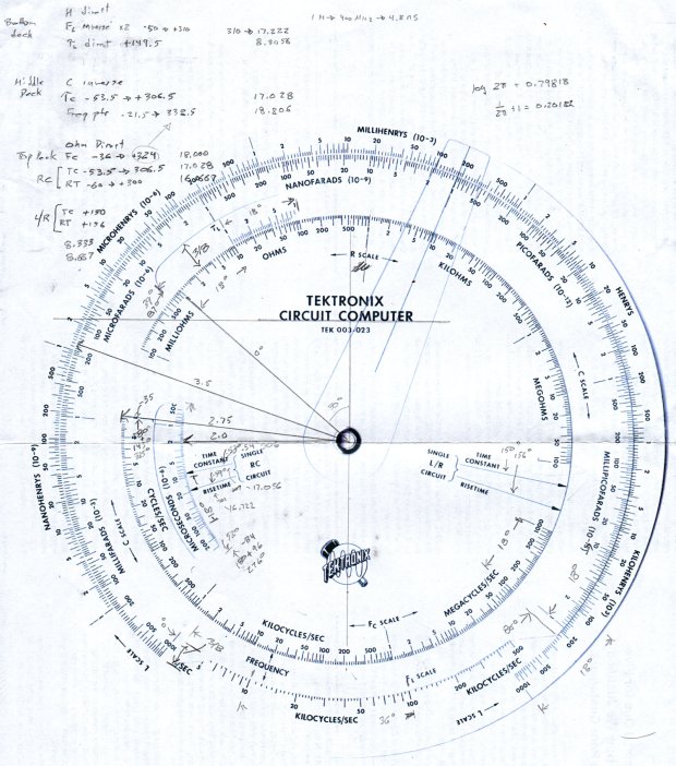
Some doodling produced key measurements:
Tektronix Circuit Computer – angle layout
All the dimensions are hard inches, of course.
Each log decade spans 18°, with the Inductive Frequency scale at 36° for the square root required to calculate circuit resonance.
Generating the log scales requires handling all possible combinations of:
Scales increase clockwise
Scales increase counterclockwise
Ticks point outward
Ticks point inward
Text reads from center
Text reads from rim
I used the 1×100 tick on the outer scale of each deck as the 0° reference for the other scales on that deck. The 0° tick appears at the far right of plots & engravings & suchlike.
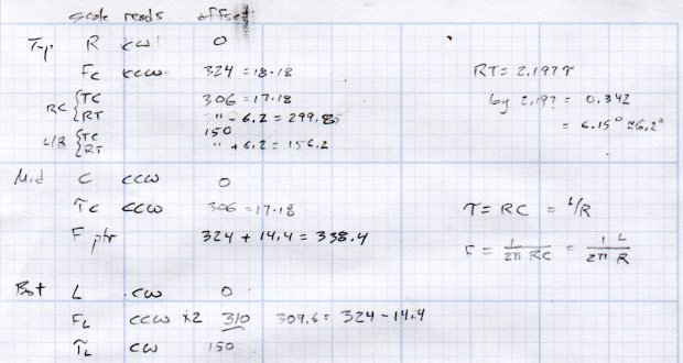
The L/R Time Constant (tau = τ) pointer on the top deck and the corresponding τL scale on the bottom deck has (what seems like) an arbitrary -150° offset from the 0° reference.
The Inductive Frequency scale has an offset of 2π, the log of which is 0.79818 = 14.37°.
The risetime calculations have a factor of 2.197, offsetting those pointers from their corresponding τ pointer by 0.342 = log(2.197) = 6.15°.
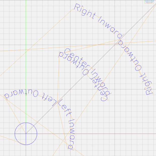
A fair bit of effort produced a GCMC program creating a full-size check plot of the bottom deck on the MPCNC:
By the conservation of perversity, the image is rotated 90° to put the 1 H tick straight up.
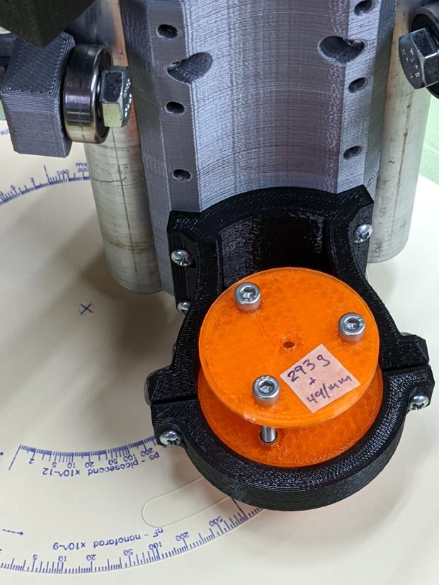
The 3018 can’t handle a 7.75 inch = 196 mm disk, but a CD-size (120 mm OD) engraving came out OK on white plastic filled with black crayon:
Tek CC bottom – ABS 160g 2400mm-min
The millimeter scale over on the right shows the letters stand a bit under 1 mm tall. And, yes, the middle scale should read upside-down.
Properly filling the engraved lines remains an ongoing experiment. More downforce on the diamond or more passes through the G-Code should produce deeper trenches, perhaps with correspondingly higher ridges along the sides. Sanding & polishing the plastic without removing the ink seems tedious.
The Great Dragorn of Kismet observes I have a gift for picking projects at the cutting edge of consumer demand.
More doodles while figuring the GCMC code produced a summary of the scale offsets:
It turned out easier to build vectors of tick mark values and their corresponding lengths, with another list of ticks to be labeled, than to figure out how to automate those values.
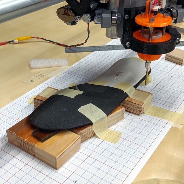
I set up an orthotic shoe insert on the MPCNC and unleashed the Z-Axis height probe on it:
Orthotic – bottom probing
In principle, the grid keeps the object aligned with the machine axes and the blocks put the upper surface more-or-less parallel with the platform. The XY origin, at the G28 location I’ve been using for tool changes, is on the midline of the sole, with Z touched off by probing the platform beside the sole.
The only interesting part of the orthotic is the rigid white plastic plate, which extends about 20 mm into a pocket in the black foam, so the probe area excludes the bendy part.
I’m abusing the bCNC Auto-level probe routine to get the height map, because it produces a tidy file of XYZ coordinates with three header lines describing the overall probe area:
The first two lines give the X and Y coordinate ranges and number of samples. The third line is the Z axis range and probe speed (?). After that, it’s just probed XYZ coordinates, all the way down.
Meshlab can import ASC files consisting of XYZ coordinates, with the ability to skip a specific number of header lines:
Meshlab ASC file import – header lines
If you don’t skip those three lines, then you get three additional points, far off in XYZ space, that will confuse the next step.
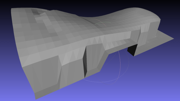
Checking the Grid Triangulation box (the default) produces a nicely lofted sheet:
Orthotic – R bottom triangulated
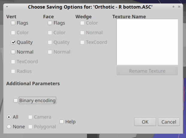
It is, however, a single-sided sheet, not a manifold 3D object. After a few days of screwing around, I’m unable to find any (automatic, reliable, non-manual) way to solidify the thing in Meshlab, so just save it as a PLY file in ASCII format:
Import it into Meshmixer, Ctrl-A to select the whole thing, click (Select →) Edit → Extrude, pick Y-Axis and Flat EndType, then extrude a convenient base in the negative direction:
Meshmixer – Y-Axis extrusion
For whatever reason, some 3D programs show machine-tool coordinates with Z pointing upward and others aim the Z axis at your face. Both must have made sense at the time, because Meshmixer defaults to swapping the Y and Z coordinates on import / export.
The Density slider controls the number of generated faces in the extruded section, so tune for best results.
I have no idea what Harden does.
Accept the result and you have a solid object suitable for further modeling.
The Poughkeepsie Library makes a 3DSystems Sense scanner (V1) available to patrons and, after a bit of to-and-fro, I managed to get a not-awful scan of Mary’s right leg:
Mary – R foot – complete
This was accomplished under field conditions in a cramped room hosting a Spanish-language “introduction to computers” class. We propped her leg across the edge of a table with her sock as a cushion.
The depth image resolution seems to be 1 mm and the software attempts to stitch multiple views from different angles into a consistent 3D model. The scanner requires a steady hand and a steady model to successfully glue new data onto the existing model; what seem small misalignments derail the matching.
The software has several presets, of which “Head” produces the best results. I have no idea what the algorithm thinks of her foot; maybe it’s been trained on some truly ugly faces.
Exporting the solid model as either STL or PLY allows import into (Windows-only) Meshmixer, wherein I sawed off the pieces we won’t need:
Mary R foot trimmed
If only I had a foot fetish …
The 3DSystems software requires a fairly specific Windows 8 (or 10, which is so not happening) + Intel hardware configuration, which recently arrived as a $250 off-lease Dell Latitude 7250 laptop. It works fine through VNC, so I can use it from the Comfy Desk.
However, using a 3D scanner in your own home isn’t actually private:
3D Systems may also automatically collect and report back to 3D Systems information about the Software and Licensee’s usage along with limited information about the Device, 3D Printer, and/or other third-party applications. If 3D Systems implements automated data collection practices then Licensee may opt out of providing such data if Licensee has a license that authorizes Commercial Use.
Oh, and then you must activate the software before using it. The library IT folks tell me I can install & activate the scanner on my system without derailing their setup. I have my doubts, but we’ll see how it goes.