Ed Nisley's Blog: Shop notes, electronics, firmware, machinery, 3D printing, laser cuttery, and curiosities. Contents: 100% human thinking, 0% AI slop.
Category: Science
If you measure something often enough, it becomes science
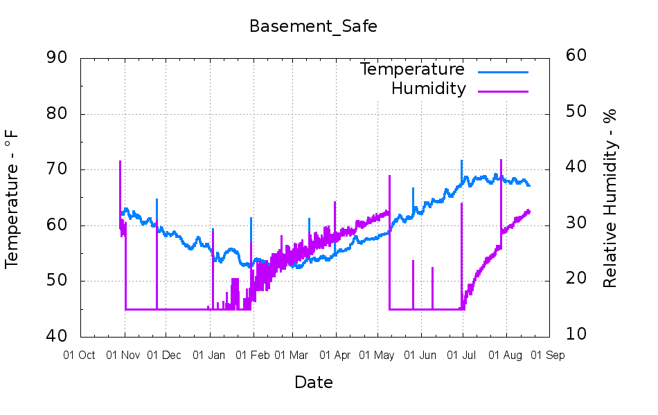
The desiccant definitely lasts longer during the winter, even though the dehumidifier fights the basement air to a standstill around 55%RH during the summer.
Each desiccant bag contains 500 g of silica gel and the most recent one adsorbed 73 g of water.
A Squidwrench Weekly Doings being useful for short-attention-span projects, I measured the DC current gain for all five ET227 transistors. The test conditions fall far below the ET227’s 1 kV / 100 A ratings, but they’re roughly what the sewing machine motor controller calls for.
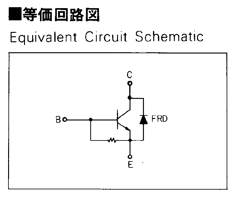
The transistors don’t even begin to turn on until IB gets over about 50 mA, because there’s a 13 Ω shunt resistor (as measured, for either polarity) between the base and emitter terminal:
Fuji ET227 – equivalent circuit
In the ET227’s normal use, that resistor dumps the Miller effect charge injected from the collector (with the intent of improving the switching time), but you must ram nearly 70 mA into the resistor to get 900 mV at the base, so the actual transistor base current isn’t all that high for low collector currents. But you measure gain by dividing goes-outa by goes-inta, so that’s what I’ll do.
The ET227 needs something like IB = 30 A to switch 100 A at the collector, so a few dozen mA into that resistor rounds off to zilch for its usual driver circuit. FWIW, with IB = 30 A, VBE tops out at 2 V: the resistor carries 150 mA and dissipates 300 mW.
Anyhow, randomly labeling the transistors from A (on the heatsink) through E, then hitching them up to a 1.8 A bench supply with a 33 Ω resistor to the base terminal provided some readings at single-digit collector voltages.
For IB = 72 mA:
IB
IC
hFE
A
72
490
6.8
B
73
540
7.4
C
74
480
6.5
D
75
440
5.9
E
76
520
6.8
For IB = 108 mA, with one bumped-knob outlier:
IB
IC
hFE
A
108
1220
11.3
B
101
1190
11.8
C
108
1280
11.9
D
108
1170
10.8
E
108
1320
12.2
Although the gain around 1 A comes out slightly higher than while running the motor, it’s in the same ballpark. This is not a high-gain device: it’ll need a driver after the optoisolator to squeeze enough current through the collector.
Eks tried to unload a huge old Tek transistor curve tracer on me that would be ideal for this sort of thing. I’m still not tempted…
I’d have trouble faking this with a straight face:
FT82-43 – 56 turns – 24 AWG
That’s measured with the 56 turn winding connected directly to a bench power supply, cranking up the current, taking the reading, and turning the current back down again, so as to avoid cooking the poor thing inside its PLA armor:
FT82-43 toroid – mounted
The “49E” sensor came from one of the bags of eBay fallout. They saturate around 4.25 V; the outputs above 4 V lose their linearity due to the sensor, not ferrite saturation.
The original calculations guesstimates suggested 25 turns would produce full scale at 5 A, so 56 turns should top out at 2.2 A. Frankly, given all the imponderables in this lashup, a factor of two seems pretty close.
Offsetting the output by -1 A would yield a 2 A range that’s just about exactly right. Unfortunately, some fiddling about with neodymium magnets suggests that you (well, I) can’t stuff enough opposing field into the slit without saturating (some part of) the ferrite core, reducing the permeability, and blowing all the assumptions.
So that suggests a buck winding, obviously with more turns to allow less current for the same magnetizing force. Wrapping 110 turns reduces the buck current to 500 mA and assuming a bit over an inch/turn requires 10 feet, which is nearly 1 Ω of 30 AWG wire: the buck current dumps another 250 mW into (a somewhat larger version of) that PLA armor.
Or just throw away half of the Hall effect sensor range and use an op amp along the lines of the LED current sensor.
I didn’t bring the HDR-AS30V camera along on the Hudson River ride, simply because each battery lasts about 1.5 hr in 1920×1080 @ 60 fps mode and I wasn’t up to replacing batteries during the ride, then charging all three every evening. Obviously, the camera wasn’t intended for that use case.
Somewhat surprisingly, the Wasabi batteries deliver the same continuous run time as the Sony battery: 1:30 vs 1:33. I used 250 mA for those discharge curves, but I think something around 500 mA would better match the camera load.
I’m sorely tempted to drill a hole in the camera’s case and wire in a honkin’ big prismatic lithium cell.
The motor winding resistance limits the peak current to about 200 V / 40 Ω = 5 A, in the absence of the transistor current limiter, and, if it gets above that, things have gone very, very wrong. Mostly, I expect currents under 1 A and it may be useful to reduce the full scale appropriately.
The cheap eBay “SS49” Hall effect sensors I’m using produce anywhere between 0.9 and 1.8 mV/G; I’ll use 1.4 mV/G, which is at least close to the original Honeywell spec. That allows a bit over ±1000 G around the sensor’s VCC/2 bias within its output voltage range (the original datasheet says minimum ±650 G), so I’ll use B = 1000 G as the maximum magnetic flux density. The overall calibration will be output voltage / input current and I’m not above doing a one-off calibration run and baking the constant into the firmware.
The effective mean path length turns out to be a useful value for a slit toroid:
effective MPL = (toroid MPL - air gap length) + (µ · air gap length)
The SS49 style sensor spec says they’re 1.6 mm thick, and the saw-cut gaps run a bit more, but 1.5 mm will be close enough for now.
The relation between all those values:
B = 0.4 π µ NI / (effective MPL)
Solving for NI:
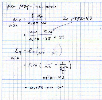
NI = B · (eff MPL) / (0.4 π µ)
Solving for N:
N = B · (eff MPL) / (0.4 π µ I)
You always round up the result for N, because fractional turns aren’t a thing you can do with a toroid.
The saturation flux density seems to be measured at H = 10 Oe, but that applies to the intact toroids. The air gap dramatically reduces the effective µ, so you must apply a higher H to get the same B in the ferrite at saturation. At least, I think that’s the way it should work.
H = 0.4 π NI / (geometric MPL)
Then:
FT50-61: H = 58 Oe
FT82-43: H = 30 Oe
I’m surely missing some second-order effect that invalidates all those numbers.
Figuring the wire size for the windings:
FT50:
ID = 0.281 inch
Circumference = 0.882 inch
28 turns → wire OD = 0.882/28 = 31 mil
20 AWG without insulation
FT82:
ID = 0.520 inch
Circumference = 1.63 inch
25 turns → wire OD = 1.63/25 = 65 mil
14 AWG without insulation
Of course, the wire needs insulation, but, even so, the FT82 allows a more rational wire size.
Page 4.12 of the writeup from Magnetics Inc has equations and a helpful chart. They suggest water cooling a diamond-bonded wheel during the slitting operation; my slapdash technique worked only because I took candy-ass cuts.
Mary signed up for the National Bike Challenge and is currently ranked 4201 out of 32 k riders, by simply getting on the damn bike and riding. About 3/4 of her miles count as “transport”: grocery / gardening / shopping / suchlike. We’re no longer biking to work, but when we did, riding ten miles a day, every day, added up pretty quickly; we chose houses in locations that made bicycle commuting possible.
Her father, at age 84, also signed up and ranked neck-and-neck with her until cataract surgery cut into his riding schedule; their standings flip-flopped depending on who updated most recently. He’s our role model for getting old without slowing down.
I’m not participating, being far more quantified than anyone really should be.
Makes you wonder what the bottom 28 k (*) riders are doing, doesn’t it? I mean, sheesh, my esteemed wife spots most participants an entire lifetime or two; her father spots them three or four. They’re not star athletes, that’s for sure, but they’re doing just fine.
(*) The Challenge had over 40 k riders at one point. We think they’ve tossed folks who haven’t done any riding at all, which might serve to improve the overall averages.
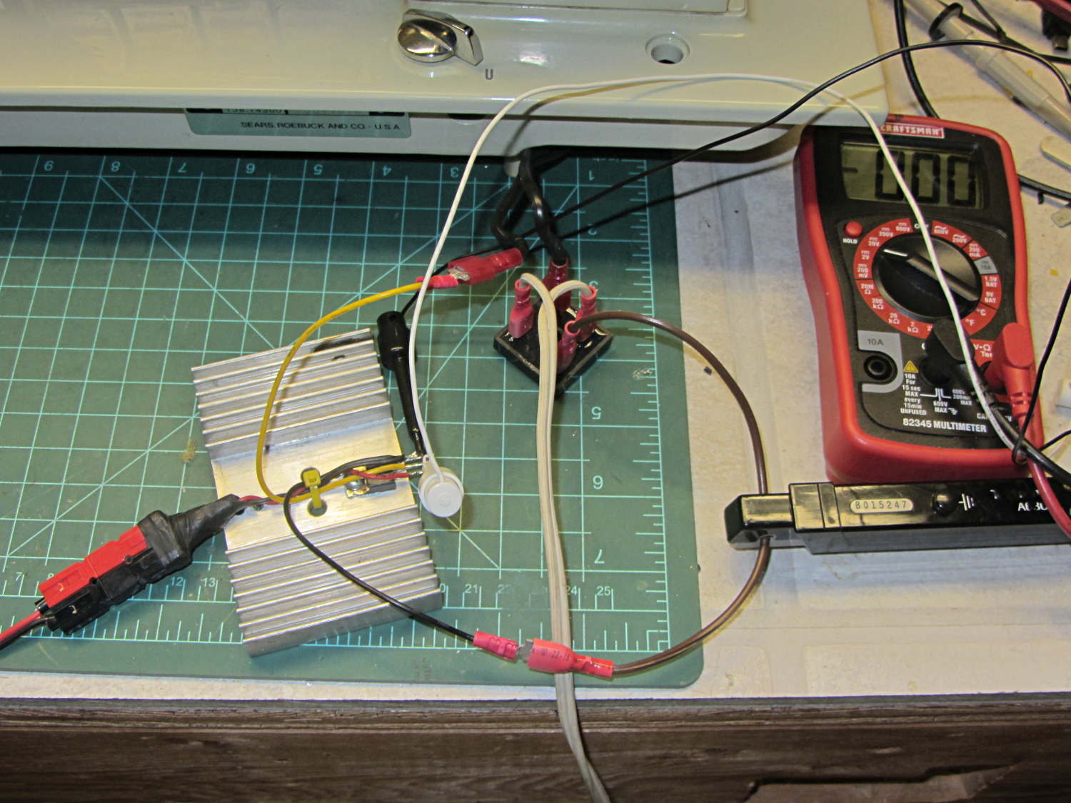
At least until I blew out the MOSFET, which is about what I expected. It’s screwed to that randomly selected heatsink, with a dab of thermal compound underneath.
Incoming AC from an isolated variable transformer (basically, an isolated Variac) goes to a bridge rectifier. Rectified output: positive to the motor, motor to MOSFET drain, MOSFET source to negative.
MOSFET gate from bench supply positive and supply negative to source.
Hall effect current probe clamped around the motor current path.
The MOSFET was an IRF610: 200 V / 3.3 A. That’s under-rated for what I was doing, but I had a bunch of ’em.
I actually worked up to that mess, starting with the bare motor on the bench running from the 50 VDC supply. That sufficed to show that you can, in fact, control the motor speed by twiddling the gate voltage to regulate the current going into the motor. It also showed that a universal-wound motor’s square-law positive feedback loop will definitely require careful tuning; think of an unstable fly-by-wire airplane and you’ve got the general idea.
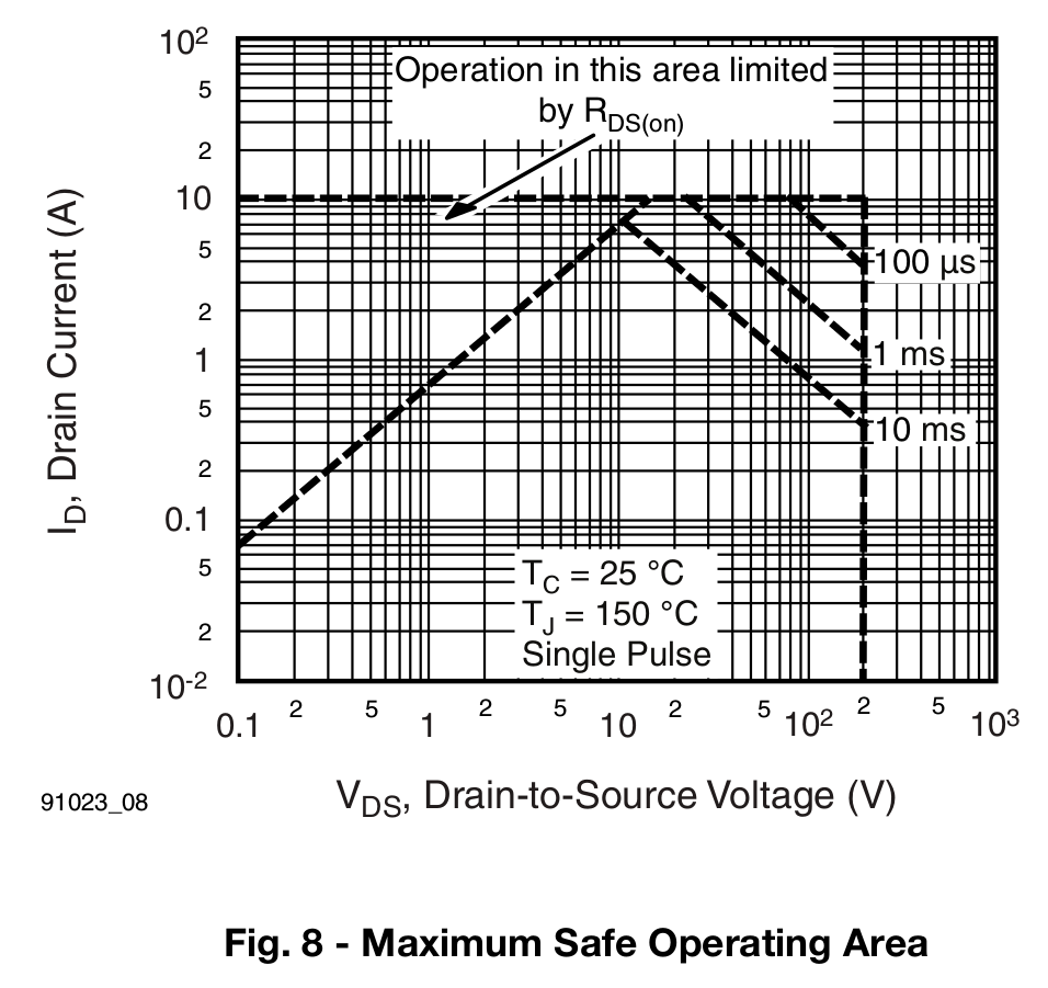
In any event, flushed with success, I ignored the safe operating area graph (from the Vishay datasheet):
IRF610 – Safe Operating Area
Drain current over half an amp at 160-ish peak volts (from rectified 120 VAC) will kill the MOSFET unless you apply it as short single pulses, not repetitive 120 Hz hammerblows.
I also ignored the transfer characteristics graph:
IRF610 – Typical Transfer Characteristics
The curve starting at the lower left should be labeled 25 °C and the other should be 150 °C. The key point is that they cross around VGS = 6.5 V, where IDS = 2 A. Below that point, the MOSFET conducts more current as it heats up… which means that if a small part of the die heats up, it will conduct more current, heat up even more, and eventually burn through.
Yes, MOSFETs can suffer thermal runaway, too.
The motor draws about half an amp while driving the sewing machine, which suggests the gate voltage will be around 5 V. In round numbers, it was 5.5 to 6 V as I twiddled the knob to maintain a constant speed.
At half an amp, the MOSFET dissipated anywhere from a bit under 1 W (from RDS(on) = 1.5 Ω to well over 25 W (while trying to maintain headway with friction on the handwheel). I ran out of fingers to record the numbers, but dropping 10 to 20 V across the MOSFET seemed typical and that turns into 5 to 10 W.
It eventually failed shorted and the sewing machine revved up to full speed. Sic transit gloria mundi.
In any event, I think the only way to have a transistor survive that sort of abuse is to start with one so grossly over-rated that it can handle a few amps at 200 V without sweating. It might actually be easier to get an ordinary NPN transistor with such ratings; using a hockey puck IGBT or some such seems like overkill.