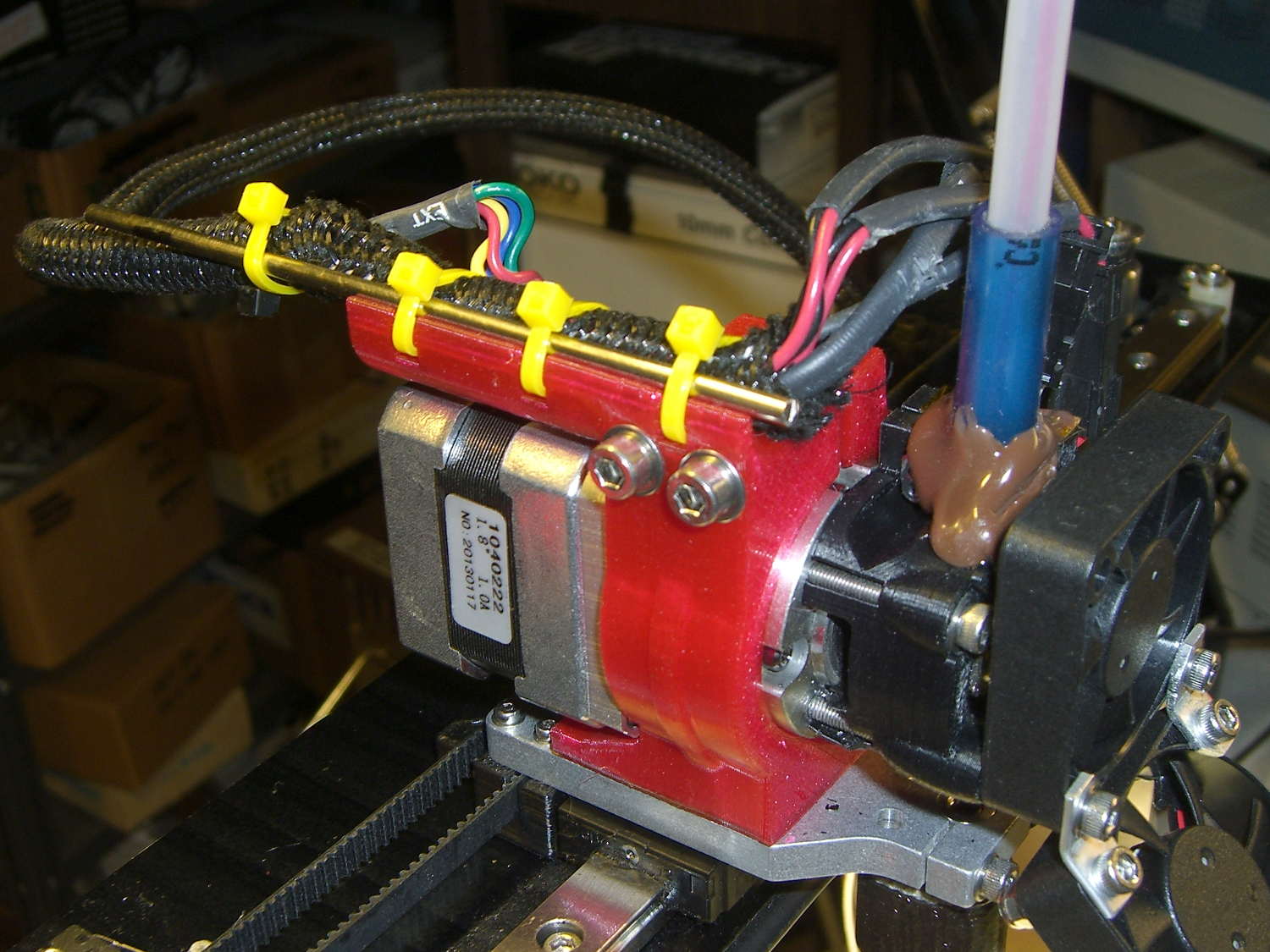
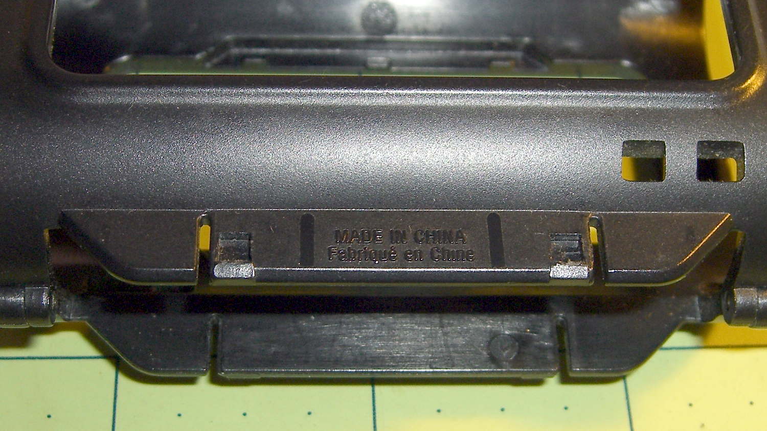
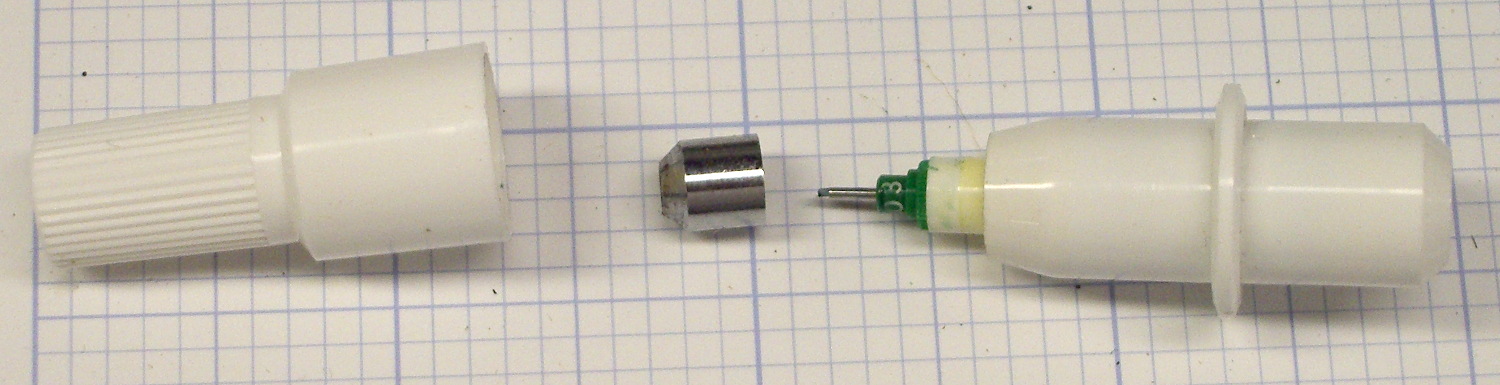
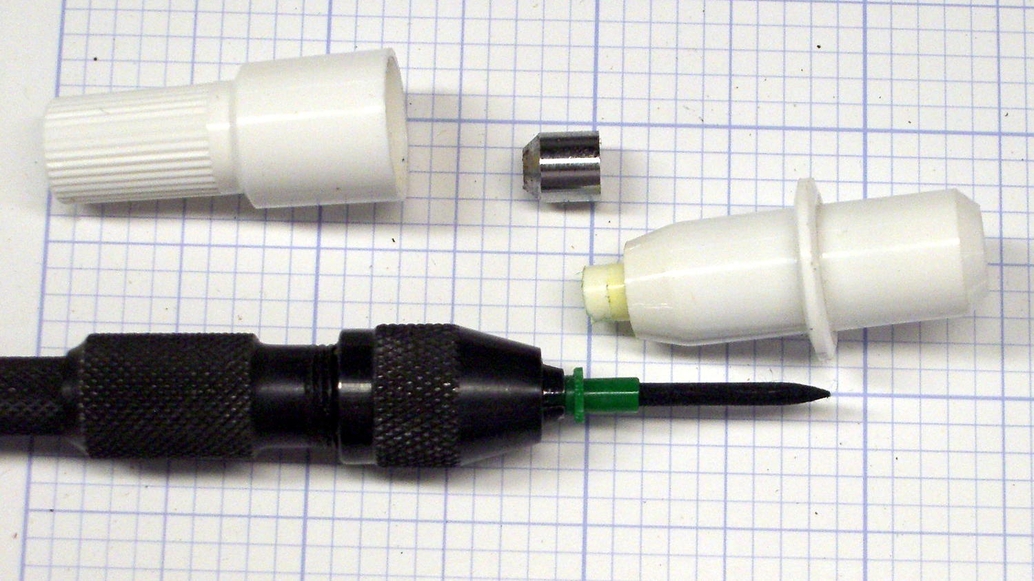
Mary flattens seam allowances and prepares appliqué pieces with a Clover MCI-900 Mini Iron. The stand resembles the wire gadgets that came with soldering irons, back in the day:

That stand may be suitable on a workbench, but it’s perilously unstable on an ironing board. After fiddling around for a while and becoming increasingly frustrated with it, she asked for a secure holder that wouldn’t fall over and perhaps had a heat shield around the hot end.
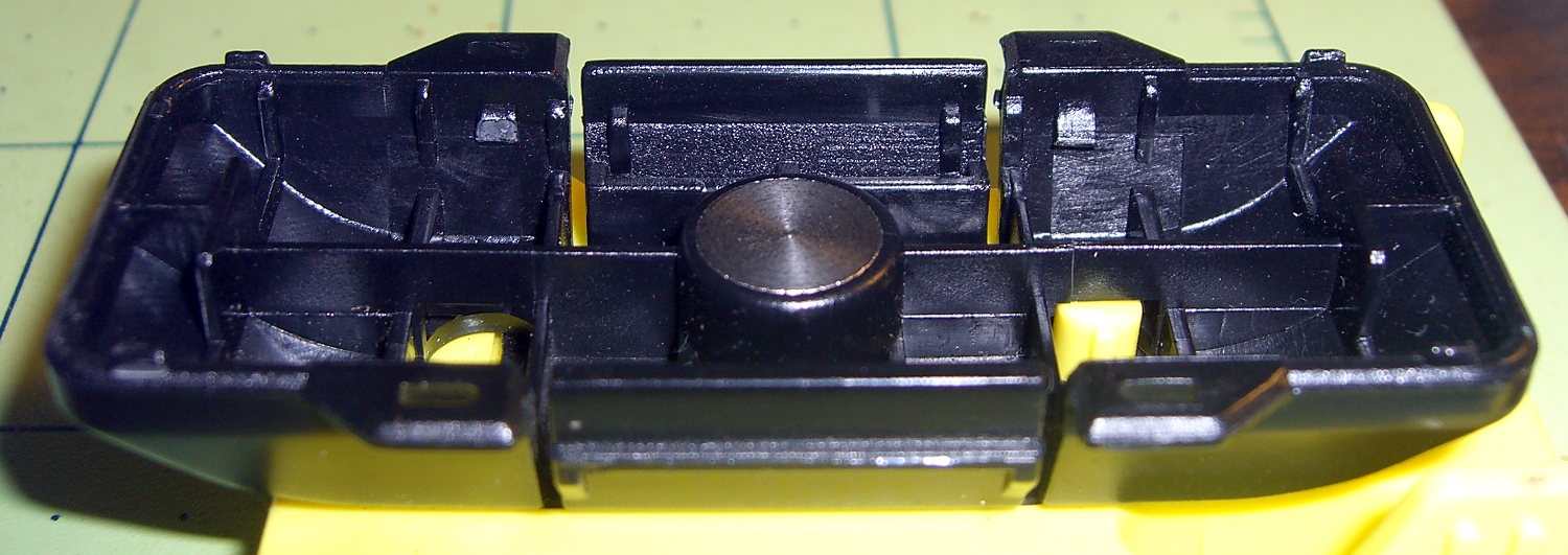
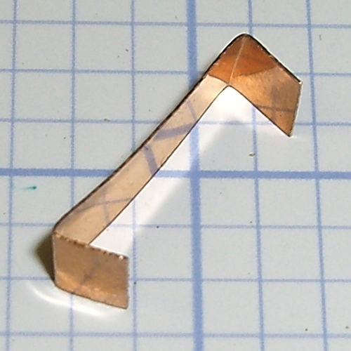
I ran off a quick prototype to verify my measurements and provide a basis for further discussion:

I proposed screwing that holder to a rectangle of leftover countertop extending under the hot end, with a U-shaped heat shield extending upward to keep fingers and fabric away from the blade. She decided the countertop might be entirely too heavy and the heat shield might be too confining, so she suggested just angling the iron upward and adding a flat platform to stabilize it.
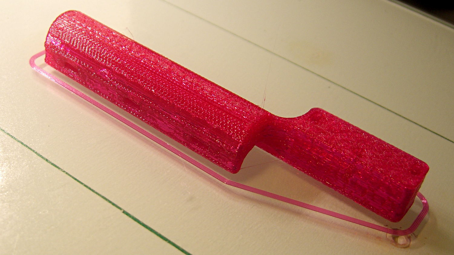
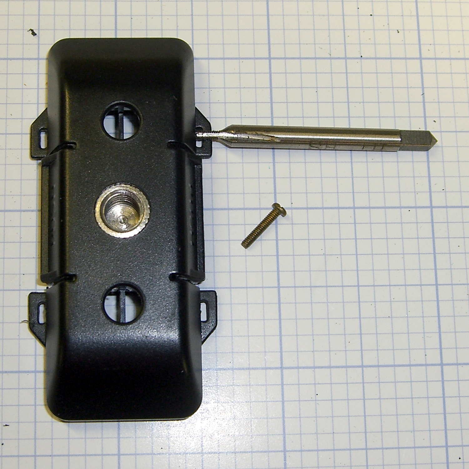
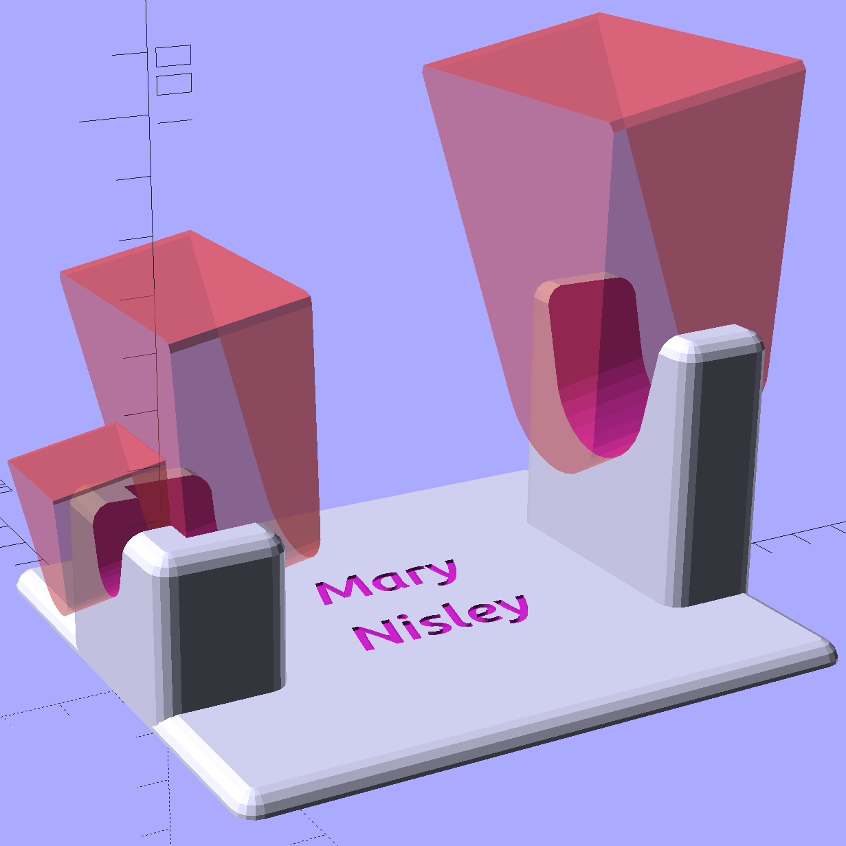
Her wish being my command:

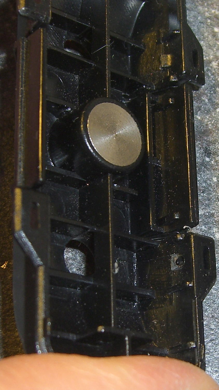
I’m still not convinced that having the hot end up in the air is a Good Thing, but she thinks it’s worth trying as-is. A pair of 10-32 screw holes under each end will let it mount to a base board, should that becomes necessary.
I’ll stick a foam sheet under the platform so it doesn’t slide around. The cord normally dangles downward off the side of the ironing board or work table, so the iron won’t get up and walk away, but it might pull the whole affair toward the edge.
Because OpenSCAD now includes a text() function, engraving her name in the platform turned out to be no big deal:

I should fill the letters with JB Weld epoxy darkened with laser printer toner (who knew?) to make them stand out. They’re more conspicuous in person than in the picture, so maybe it doesn’t matter.
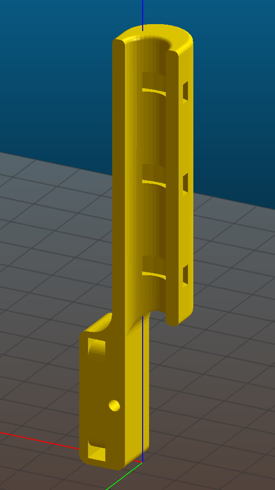
The slots holding the iron have a semicircular bottom and straight-wall sides, created by extruding hulled 2D shapes, arranging them along the iron’s central axis, and tilting the “iron” at the appropriate angle:
That’s a 10° tilt, chosen because it looked right. The model recomputes itself around the key dimensions, so we can raise / lower the iron, change the angle, and so forth and so on, as needed.
Assuming that a hot end sticking out in mid-air isn’t too awful, this one looks like a keeper.
The OpenSCAD source code:
// Clover MCI-900 Mini Iron holder
// Ed Nisley KE4ZNU - August 2015

Layout = "Holder";					// Iron Holder

//- Extrusion parameters - must match reality!

ThreadThick = 0.25;
ThreadWidth = 0.40;

function IntegerMultiple(Size,Unit) = Unit * ceil(Size / Unit);

Protrusion = 0.1;

HoleWindage = 0.2;

inch = 25.4;

Tap10_32 = 0.159 * inch;
Clear10_32 = 0.190 * inch;
Head10_32 = 0.373 * inch;
Head10_32Thick = 0.110 * inch;
Nut10_32Dia = 0.433 * inch;
Nut10_32Thick = 0.130 * inch;
Washer10_32OD = 0.381 * inch;
Washer10_32ID = 0.204 * inch;

//------
// Dimensions

CornerRadius = 4.0;

CenterHeight = 25;							// center at cord inlet on body

BodyLength = 110;							// cord inlet to body curve at front flange

Incline = 10;								// central angle slope

FrontOD = 29;
FrontBlock = [20,1.5*FrontOD + 2*CornerRadius,FrontOD/2 + CenterHeight + BodyLength*sin(Incline)];

CordOD = 10;
CordLen = 10;

RearOD = 22;
RearBlock = [15 + CordLen,1.5*RearOD + 2*CornerRadius,RearOD/2 + CenterHeight];

PlateWidth = 2*FrontBlock[1];

TextDepth = 3*ThreadThick;

ScrewOC = BodyLength - FrontBlock[0]/2;
ScrewDepth = CenterHeight - FrontOD/2 - 5;

echo(str("Screw OC: ",ScrewOC));

BuildSize = [200,250,200];					// largest possible thing

module PolyCyl(Dia,Height,ForceSides=0) {			// based on nophead's polyholes

  Sides = (ForceSides != 0) ? ForceSides : (ceil(Dia) + 2);

  FixDia = Dia / cos(180/Sides);

  cylinder(r=(FixDia + HoleWindage)/2,
           h=Height,
	   $fn=Sides);
}

// Trim bottom from child object

module TrimBottom(BlockSize=BuildSize,Slice=CornerRadius) {

	intersection() {
		translate([0,0,BlockSize[2]/2])
			cube(BlockSize,center=true);
		translate([0,0,-Slice])
			children();
	}
}

// Build a rounded block-like thing

module RoundBlock(Size=[20,25,30],Radius=CornerRadius,Center=false) {

	HS = Size/2 - [Radius,Radius,Radius];
	translate([0,0,Center ? 0 : (HS[2] + Radius)])
	hull() {
		for (i=[-1,1], j=[-1,1], k=[-1,1]) {
			translate([i*HS[0],j*HS[1],k*HS[2]])
				sphere(r=Radius,$fn=4*4);
		}
	}
}

// Create a channel to hold something
// This will eventually be subtracted from a block
// The offsets are specialized for this application...

module Channel(Dia,Length) {

	rotate([0,90,0])
		linear_extrude(height=Length)
			rotate(90)
				hull() {
					for (i=[-1,1])
						translate([i*Dia,2*Dia])
							circle(d=Dia/8);
					circle(d=Dia,$fn=8*4);
				}
}

// Iron-shaped series of channels to be removed from blocks

module IronCutout() {

	union() {
		translate([-2*CordLen,0,0])
			Channel(CordOD,2*CordLen + Protrusion);
		Channel(RearOD,RearBlock[0] + Protrusion);
		translate([BodyLength - FrontBlock[0]/2 - FrontBlock[0],0,0])
			Channel(FrontOD,2*FrontBlock[0]);

	}

}

//- Build it

if (Layout == "Iron")
	IronCutout();

if (Layout == "Holder")
	difference() {
		union() {
			translate([(BodyLength + CordLen)/2 - CordLen,0,0])
				TrimBottom()
					RoundBlock(Size=[(CordLen + BodyLength),PlateWidth,CornerRadius]);

			translate([(RearBlock[0]/2 - CordLen),0,0])
				TrimBottom()
					RoundBlock(Size=RearBlock);

			translate([BodyLength - FrontBlock[0]/2,0,0]) {
				TrimBottom()
					RoundBlock(Size=FrontBlock);
			}
		}

		translate([0,0,CenterHeight])
			rotate([0,-Incline,0])
				IronCutout();

		translate([0,0,-Protrusion])
			PolyCyl(Tap10_32,ScrewDepth + Protrusion,6);

		translate([ScrewOC,0,-Protrusion])
			PolyCyl(Tap10_32,ScrewDepth + Protrusion,6);

		translate([(RearBlock[0] - CordLen) + BodyLength/2 - FrontBlock[0],0,CornerRadius - TextDepth]) {

			translate([0,10,0])
				linear_extrude(height=TextDepth + Protrusion,convexity=1)		// rendering glitches for convexity > 1
					text("Mary",font="Ubuntu:style=Bold Italic",halign="center",valign="center");

			translate([0,-10,0])
				linear_extrude(height=TextDepth + Protrusion,convexity=1)		// rendering glitches for convexity > 1
				text("Nisley",font="Ubuntu:style=Bold Italic",halign="center",valign="center");
		}

	}
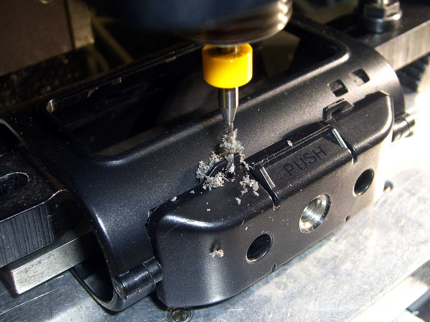
The M2 buzzed away for four hours on that puppy, with the first 2½ hours devoted to building the platform. That’s the downside of applying Hilbert Curve infill to two big flat surfaces, but the texture looks really good.