HP 7475A Plotter: Superformula Demo

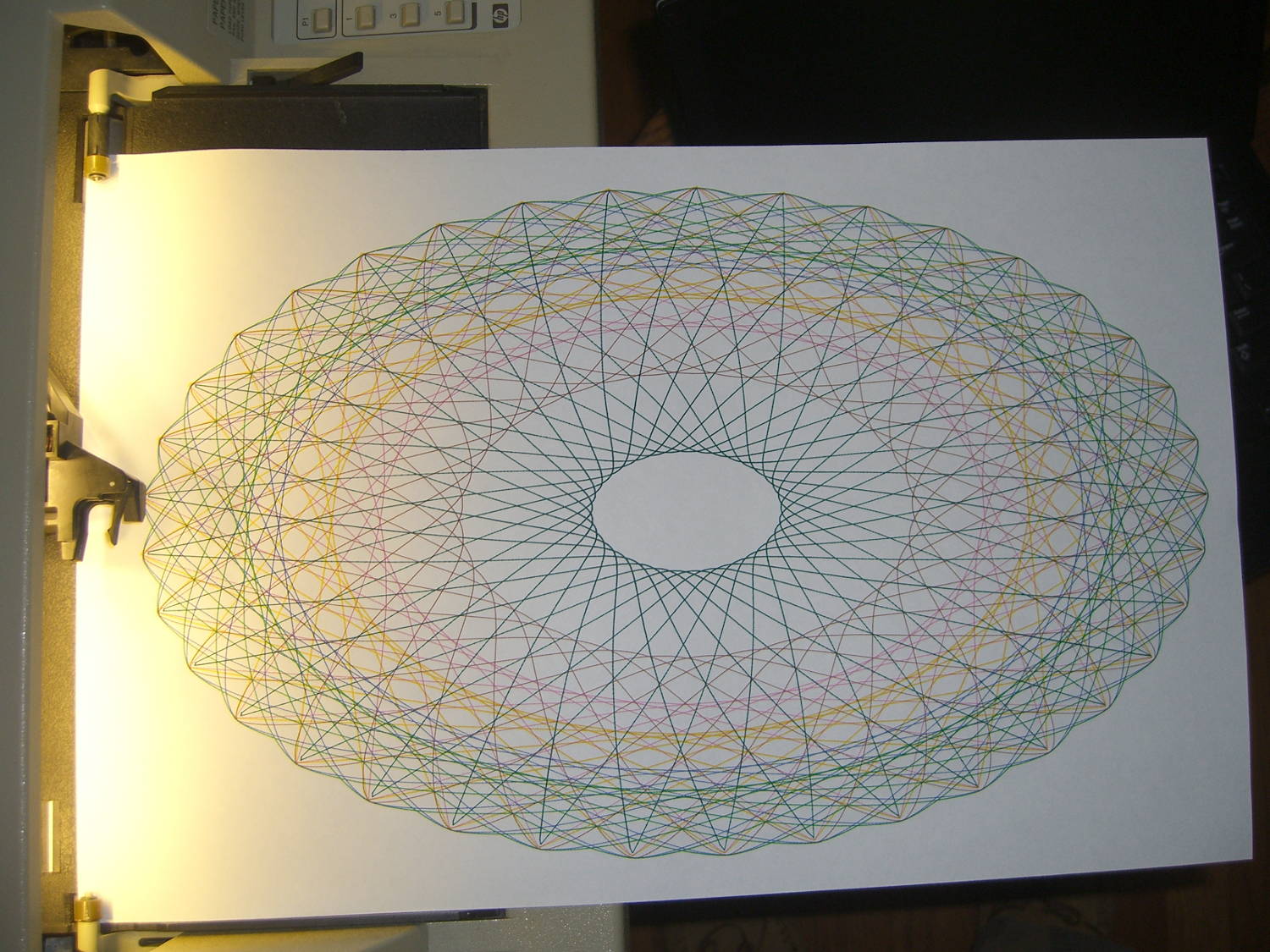
Setting n2=n3=1.5 generates smoothly rounded shapes, rather than the spiky ones produced by n2=n3=1.0, so I combined the two into a single demo routine:

A closer look shows all the curves meet at the points, of which there are 37:

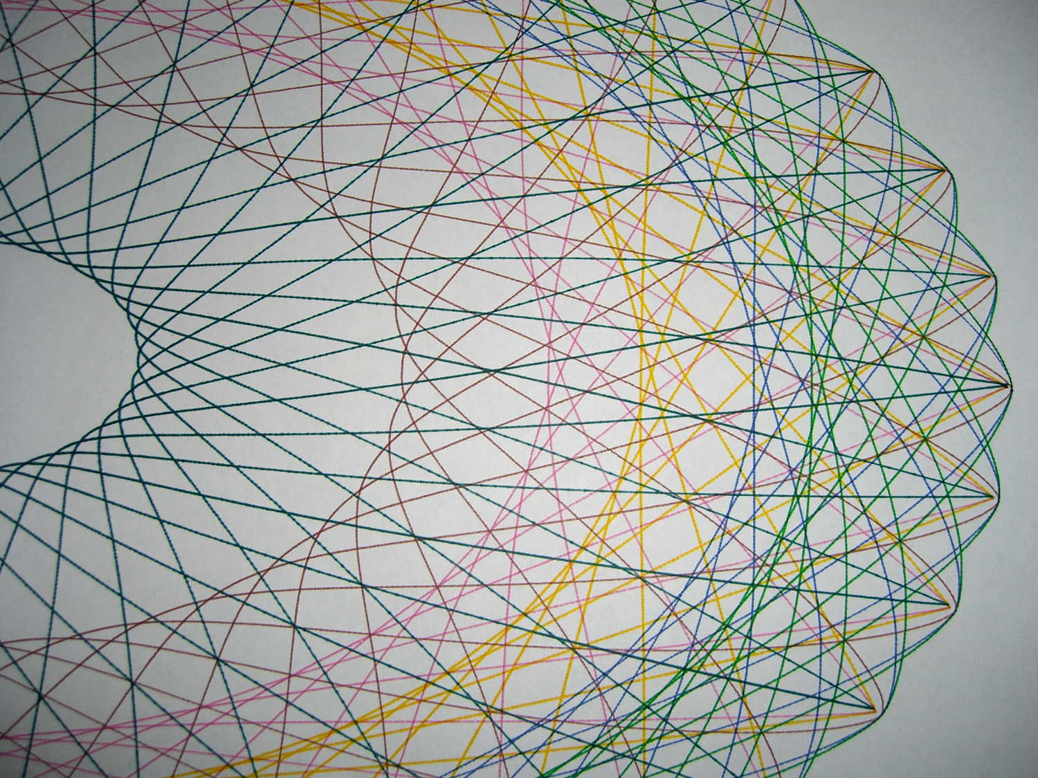
The spikes suffer from limited resolution: each curve has 10 k points, but if the extreme end of a spike lies between two points, then it gets blunted on the page. Doubling the number of points would help, although I think this has already gone well beyond the, ah, point of diminishing returns.

I used the three remaining “disposable” liquid ink pens for the spiked curves; the black pen was beyond repair. They produce gorgeous lines, although the magenta ink seems a bit thinned out by the water I used to rinse the remains of the last refill out of the spiral vent channel.

I modified the Chiplotle supershape() function to default to my choices for point_count and travel, then copied the superformula() function and changed it to return polar coordinates, because I’ll eventually try scaling the linear value as a function of the total angle, which is much easier in polar coordinates.

The demo code produces the patterns in the picture by iterating over interesting values of n1 and n2=n3, stepping through the pen carousel for each pattern. As before, m should be prime/10 to produce a prime number of spikes / bumps. You could add more iteration values, but six of ’em seem entirely sufficient.

A real demo should include a large collection of known-good parameter sets, from which it can pick six sets to make a plot. A legend documenting the parameters for each pattern, plus the date & time, would bolster the geek cred.

The Python source code with the modified Chiplotle routines:

from chiplotle import *
from math import *

def superformula_polar(a, b, m, n1, n2, n3, phi):
   ''' Computes the position of the point on a
   superformula curve.
   Superformula has first been proposed by Johan Gielis
   and is a generalization of superellipse.
   see: http://en.wikipedia.org/wiki/Superformula
   Tweaked to return polar coordinates
   '''

   t1 = cos(m * phi / 4.0) / a
   t1 = abs(t1)
   t1 = pow(t1, n2)

   t2 = sin(m * phi / 4.0) / b
   t2 = abs(t2)
   t2 = pow(t2, n3)

   t3 = -1 / float(n1)
   r = pow(t1 + t2, t3)
   if abs(r) == 0:
      return (0,0)
   else:
 #     return (r * cos(phi), r * sin(phi))
     return (r,phi)

def supershape(width, height, m, n1, n2, n3,
   point_count=10*1000, percentage=1.0, a=1.0, b=1.0, travel=None):
   '''Supershape, generated using the superformula first proposed
   by Johan Gielis.

   - `points_count` is the total number of points to compute.
   - `travel` is the length of the outline drawn in radians.
      3.1416 * 2 is a complete cycle.
   '''
   travel = travel or (10*2*pi)

   ## compute points...
   phis = [i * travel / point_count
      for i in range(1 + int(point_count * percentage))]
   points = [superformula_polar(a, b, m, n1, n2, n3, x) for x in phis]

   ## scale and transpose...
   path = [ ]
   for r, a in points:
      x = width * r * cos(a)
      y = height * r * sin(a)
      path.append(Coordinate(x, y))

   return Path(path)

## RUN DEMO CODE

if __name__ == '__main__':
   paperx = 8000
   papery = 5000
   if  not False:
     plt=instantiate_plotters()[0]
     plt.set_origin_center()
     plt.write(hpgl.VS(10))
     pen = 1
     for m in [3.7]:
        for n1 in [0.20, 0.60, 0.8]:
          for n2 in [1.0, 1.5]:
              n3 = n2
              e = supershape(paperx, papery, m, n1, n2, n3)
              plt.select_pen(pen)
              if pen < 6:
                 pen += 1
              else:
                 pen = 1
              plt.write(e)
     plt.select_pen(0)
   else:
     e = supershape(paperx, papery, 1.9, 0.8, 3, 3)
     io.view(e)