Now that I understand why the M2 Z axis stepper gets so hot, the question is: does it matter?
The Z axis stage moves very smoothly along the two guide rails, so there’s little friction and no binding involved. I can’t weigh the thing without dismantling the whole printer, which isn’t going to happen right now, but some crude experiments indicate that 7 pounds = 3 kgf = 30 N isn’t too far from the truth.
The 8 mm OD leadscrew has a 4-start thread at 3.25 turn/inch = 0.311 inch/turn = 0.13 turn/mm = 7.8 mm/turn.
[Update: Thanks to Jetguy for pointing out the blindingly obvious fact that it’s really 8 mm/turn = 0.125 turn/mm and you can do the inch conversion yourself if you need it. That doesn’t materially affect the results, given that they have about one significant figure of accuracy to start with.]
The firmware uses 1/16 microstepping at 400 step/mm = 3077 3200 step/turn.
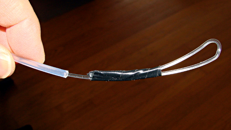
Using a pull scale to, yes, pull a string wound around the knob on the Z axis leadscrew shows about 1 pound raises the platform at a slow, constant speed. The polygonal knob is about 35 mm in diameter, so the torque works out to 11 ounce·inch = 80 mN·m. Presumably, holding the platform at a given position would require somewhat less torque, but I can’t measure that with any confidence.
The motor has very little excess torque: a gentle touch can stall the Z axis motor as it raises the stage. I guesstimate the motor produces 150 mN·m, tops, during low-speed motion at 600 mA.
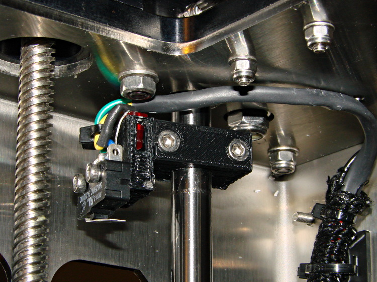
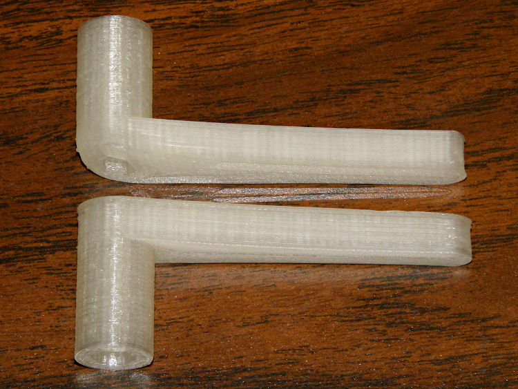
Lowering the stage requires no effort at all: it falls under its own weight, prompting me to install those bumpers. The design doesn’t have much compliance, but it’s well-adjusted and works fine.
Searching with the appropriate keywords produces a 17HD-B8X300-H motor from Kysan:
- 12 V
- 400 mA
- 30 Ω
- 42 mH
- 2.6 kg·cm = 260 mN·m
That’s a close-enough match to suggest my measurements are in the right ballpark. The extremely high resistance and inductance indicate this is the wrong motor for a high-performance microstepping application.
The firmware has DEFAULT_MAX_ACCELERATION = 30 mm/s2 for the Z axis. It’s 9000 for X and Y, 10000 for the extruder. The extremely low Z acceleration says there’s something badly wrong with this setup.
There is also a DEFAULT_ACCELERATION = 3000 for all axes. I don’t know how that interacts with the per-axis limit, but I’m certain the Z axis doesn’t come close to that value.
I do not know how the firmware actually handles motor steps while ramping up and down, but I do intend to clamp a current probe around a motor wire and measure what goes on. Let us assume it works in the usual way all ideal components behave in physics labs.
Assuming a constant 30 mm/s2 acceleration for the first half of a 0.25 mm Z axis move, the time should be:
0.25 / 2 = (1/2) * 30 * t2
t = 90 ms
At the end of that ramp-up, the Z stage will be trundling along at:
v2 = 2 * 30 * 0.25/2
v = 2.8 mm/s
The move requires exactly 50 steps = 0.25/2 mm * 400 step/mm.
Assuming the same deceleration during the second half of the move, a 0.25 mm layer change requires about twice that long: 180 ms for 100 steps.
Along the X axis, a 0.25/2 mm move requires 5.3 ms and reaches a peak speed of 47 mm/s. The total move requires 11 ms and 22.22 steps (= 0.25 mm * 88.88 step/mm, obviously rounded to 22).
I think a difference of more than an order of magnitude matters, although some actual measurements are definitely appropriate.