Ed Nisley's Blog: Shop notes, electronics, firmware, machinery, 3D printing, laser cuttery, and curiosities. Contents: 100% human thinking, 0% AI slop.
Category: Science
If you measure something often enough, it becomes science
The general idea is to cut a USB extension cable (Type A plug on one end, Type A receptacle on the other) in half, splice the two data wires, splice the ground / common wire, but connect the +5 V wires to a dual banana plug that goes into a current meter. The Big Box o’ USB Junk produced a cutoff cable end with a Type A plug and a PC jumper that was supposed to connect an internal USB header to the back panel; the red blob of silicone tape conceals the jumper’s socket strip and a five-pin male header with all the wires soldered to it.
You could use a Type B plug that would go directly into an Arduino UNO (or similar), but I figured this way everybody can bring whatever cable they need for their particular Arduino, not all of which have bulky Type B receptacles these days.
The External Power version:
External Power Current Tap
The coaxial power plug goes into the Arduino and whatever you used for power goes into the socket. The Big Box o’ Coaxial Power Stuff actually had a more-or-less properly sized coaxial jack with two wires on it and silicone tape wrapped around it; I regarded that as a Good Omen and pressed it into service as-is.
These will also replace the horribly rickety collection of alligator clip leads I usually use for such measurements…
Unlike most Arduino courses, I assume you’re already OK with the programming, but are getting tired of replacing dead Arduinos and want to know how to keep them alive. The course description says it all:
Learn how to help your Arduino survive its encounter with your project, then live long and prosper. Discover why feeding it the proper voltages, currents, and loads ensures maximum Arduino Love!
Ed will describe some fundamental electronic concepts, guide you at the workbench while you make vital measurements, then show you how to calculate power dissipation, load current, and more. You’ll understand why Arduinos get hot, what kills output bits, and how you can finally stop buying replacements.
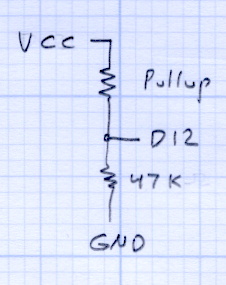
Among other lab exercises, we’ll measure the value of the ATmega’s internal pullup resistors, which everybody assumes are 20 kΩ, but probably aren’t. Hint: you can apply Ohm’s Law twice to that simple circuit and come up with the right answer, but only if you’ve measured the actual VCC voltage on the board.
The Mighty Thor will detail how to not prepare Fried Raspberry Pi.
In the unlikely event you’re in Highland NY, stop by: you’re bound to learn something.
I wound up doing an impromptu magnetics (as it applies to transformers) review during a recent SqWr meeting. This summarizes, re-orders, and maybe expands on some quadrille paper scribbling, so that if I ever do it again I’ll have a better starting point. Searching on the obvious terms will produce a surfeit of links; Wikipedia may be helpful for diagrams.
Corrections and further points-to-ponder will be gratefully received…
Magnetizing force H comes from amp-turns (amps I, turns N) around the core, which produces flux phi = Φ = NI.Edit: that’s not quite right. Thanks to Martin Bosch for catching the units mismatch!
Magnetomotive force ℱ comes from ampere-turns (amps I, turns N) around the core: mmf = ℱ = NI.
The magnetizing force H is the mmf per unit length of the solenoid or core: H = ℱ / L.
Flux density B comes from permeability (mu = μ) times H, which is a DC relationship that doesn’t care about frequency in the least: B = μH. For an air-core inductor or transformer, μ is the mu-sub-zero = μ0 of free space, but if there’s a core involved, then you use the permeability of the material near the conductor, which will be the material’s dimensionless relative permeability μR times μ0.
Total flux Φ is the integral of flux density B over all the little areas covering the surface you’re interested in, oriented in a consistent manner using the right-hand rule.
If you have an iron(-like) core inside the coil, then essentially all the flux is in the core, so the integral reduces to B times the area (call it a) of the core at right angles to the flux: Φ = Ba = μaH. In this case, μ is the relative permeability of the core times μ0 of free space.
You can plot BH curves (B for various H values) using a straightforward circuit and an oscilloscope. The X axis voltage is proportional to the winding current I and the Y axis voltage is proportional to Φ. The trick is the integrator on the secondary that converts EMF = dΦ / dt into a voltage directly proportional to Φ. The same trick works on inductors if you add a few turns to act as a secondary.
All that’s true for DC as well as AC, but transformers only work on AC, as summarized by Lenz.
The induced EMF is proportional to flux change through the secondary windings, which number n turns: EMF = – n dΦ / dt. That’s obviously proportional to frequency: higher frequency = higher EMF. Flux is all in the transformer core, so it’s still μaH. Note that these are secondary turns, so it’s n rather than N. Air-core transformers exist, but coupling the flux poses a problem; looking up variometer or variocoupler may be instructive.
The negative sign says the induced EMF creates a current that creates a magnetic field that points the other way, so as to oppose the original field change. In effect, the induced EMF works to cancel out the field you’re creating.
Knowing how much EMF you need in the secondary for the purposes of your circuit, you know the product of five things:
n – secondary turns
μ – (relative) core permeability
a – area
f – frequency
H – from primary
Now you get to pick what’s important, but they all have gotchas:
The ratio n:N seems easy to control, but it tops out at a few hundred. If you care about the voltage ratio, then that fixes the turns ratio.
Choose different core material to increase μ, but then you hit core saturation in B as H increases. Practical core materials may give you permeability over two or three orders of magnitude, but with significant side effects.
Reduce B for a given Φ by using a larger core area a, which obviously requires a bigger core that may not fit the application.
Increase frequency f to get more EMF and thus H, but it may be limited by your application and other losses and effects. Higher frequency = more traverses of that BH curve with hysteresis = more core losses = can’t use lossy metals.
Increase primary H, but again you hit core saturation in B.
The circuit driving the primary must be able to handle the total load, which means it must be able to drive the impedance presented by the transformer + secondary load. That determines the primary inductance (to get the reactance high enough that the transformer presents the secondary load to the primary circuit), which determines the core + turns at the operating frequency.
The core must support the flux required to drive the load without saturation, which constrains the material and the area. For heavy loads (i.e., “power” transformers), output power also constrains the secondary turns and wire size, which constrains the minimum core opening and thus overall size.
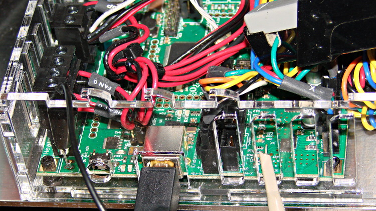
Based on the discussion attached to the post on Z axis numbers, I wanted to take a look at the points where Marlin switches from one step per interrupt to two, then to four, just to see what the timing looks like. The RAMBo board has neatly labeled test points, to which I tack-soldered a pin for the scope probe poked through one of the ventilation slots, and an unused power connector on the left edge of the PCB that provided a ground point (admittedly, much too far away for good RF grounding, but it suffices for CMOS logic signals). The Tek Hall-effect current probe leaning in from the top right captures the current in one of the X axis windings:
X axis Step and Current probes
I’ve reset the Marlin constants based on first principles, per the notes on distance, speed, and acceleration, so they’re not representative of the as-shipped M2 firmware. Recapping the XY settings:
Distance: 88.89 step/mm
Speed: 450 mm/s = 27000 mm/min
Acceleration: 5000 mm/s2, with the overall limit at 10 m/s2
The maximum interrupt frequency is about 10 kHz and the handler can issue zero, one, two, or four steps per axis per interrupt as required by the speed along each axis, up to a maximum of step rate of 40 kHz. There are complexities involved which I do not profess to understand.
The maximum 10 kHz step rate for one-step-per-interrupt motion corresponds to a speed of:
112.5 mm/s = (10000 step/s) / (88.89 step/mm)
The maximum 40 kHz step rate produces, naturally enough, four times that speed:
450 mm/s = (40000 step/s) / (88.89 step/mm)
Assuming constant acceleration, the distance required to reach a given speed from a standing start or to decelerate from that speed to a complete stop is: x = v2 / (2 * a)
The time required to reach that speed is: t = v/a
Accelerating at 5000 mm/s2:
112.5 mm/s = 6700 mm/min → 1.27 mm, 22.5 ms
150 mm/s = 9000 mm/min → 2.25 mm, 30 ms
450 mm/s = 27000 mm/min → 20.3 mm and 90 ms
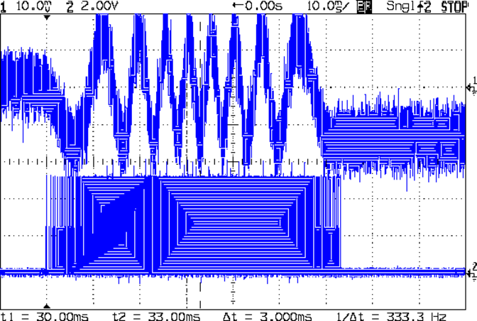
An overview of a complete 6 mm move at 150 mm/s shows the acceleration and deceleration at each end, with a constant-speed section in the middle:
X Axis 150 mm-s 6 mm – overview
The bizarre patterns in the traces come from hp2xx‘s desperate attempts to discern the meaning of the scope’s HPGL graphic data where the trace forms a solid block of color; take it as given that there’s no information in the pattern. I described the trace conversion process there.
The upper trace shows the X axis motor winding current at a scale of 500 mA/div, with far more hash than one would expect. The RAMBo drivers evidently produce much more current noise than the brick drivers I intend to use.
The lower trace is the X axis step signal produced by the Arduino microcontroller. You can barely make out the individual step signals at each end, but there’s not enough horizontal resolution to show them when the motor moves at a reasonable pace.
In round numbers, the acceleration and deceleration should require about 30 ms each. The overall move takes 63 ms, so the constant-speed section in the middle must be about 3 ms long. That’s probably not right…
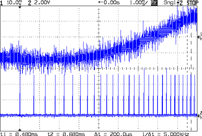
Here’s a closer look at the step pulses as the motion starts from zero on the way to 150 mm/s:
X Axis 150 mm-s 6 mm – 1 ms-div 0 ms dly
Over on the right, the 5 kHz step rate after 8.5 ms suggests a speed of 56 mm/s and counting 28 pulses says it moved 0.32 mm. Plugging those numbers into the equations:
a = v/t = 6600 mm/s2
a = (2 * x)/t2 = 8900 mm/s2
It’s not clear (to me, anyway) whether:
The firmware accelerates faster than the alleged 5000 mm/s2 limit
It’s accelerating near the overall limit of 10000 mm/s2
The acceleration isn’t constant: starts high, then declines
The measurement accuracy doesn’t support any conclusions
I understand what’s happening
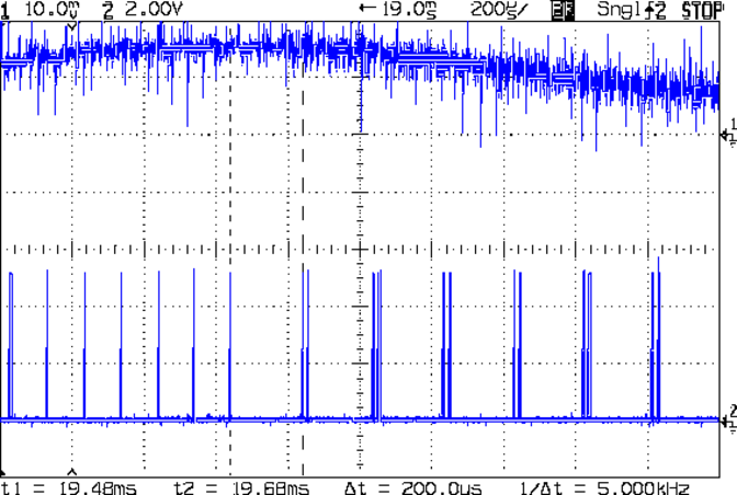
In order to see the double- and quad-step outputs, here’s a 50 mm move at 450 mm/s, with a 19 ms delay to the point where the interrupt handler transitions from single-step to double-step output:
X Axis 450 mm-s 50 mm – 200 us-div 19 ms dly
The interrupt frequency drops from just under 10 kHz to a bit under 5 kHz, with the doubled pulses about 16 μs apart. At the transition, the axis speed is 112.5 mm/s, pretty much as predicted.
If that’s the case, the overall acceleration to the transition works out to:
5800 mm/s2 = (113 mm/s) / (19.5 ms)
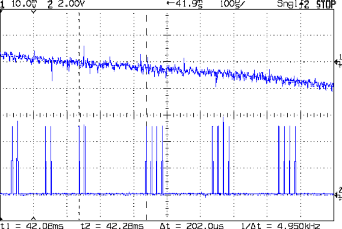
Delaying the traces to 41.9 ms after the motion starts shows the double-to-quad step transition:
X Axis 450 mm-s 50 mm – 100 us-div 41.9 ms dly
Once again, the pulse frequency drops from 10 kHz down to 5 kHz. The speed is now 225 mm/s, half the maximum possible speed, which also makes sense: at top speed, the pulses will be essentially continuous at 40 kHz.
The average acceleration from the start of the motion:
5300 mm/s2 = (225 mm/s) / (42.1 ms)
That implies the initial acceleration starts higher than the limit, but it evens out on the way to the commanded speed.
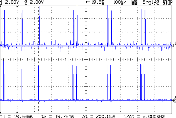
Those scope shots come from moving only the X axis. Moving both the X and Y axes, with Trace 1 now showing the Y axis output, for 50 mm at 450 mm/s, produces similar results; the Y axis output lags the X axis by a few microseconds:
XY 450 mm-s 50 mm – 100 us-div 19.5 ms dly
Once again, that’s at the single- to double-step transition at 19+ ms. The overall timing doesn’t depend on how many axes are moving, as long as they can accelerate at the same pace; otherwise, the firmware must adjust the accelerations to make both axes track the intended path.
None of this is too surprising.
For a motor running at a constant speed just beyond the single-to-double step transition at 112.5 mm/s or the double-to-quad transition at 225 mm/s, the rotor motion should have a 5 kHz perturbation around its nominal position: it coasts for nearly the entire period, then a pair of steps kicks it toward the proper position. At those transitions, the rotor turns at:
The perturbation should look like a 5 kHz oscillation (not exactly sinusoidal, maybe triangular?) superimposed on the nominal position, which is changing more-or-less parabolically as a function of time. I expect that the overall inertia damps it out pretty well, but I’d like to attach a rotary encoder to the motor shaft (or a linear encoder to the axis) to show the actual outcome, but I don’t have the machinery for that.
In any event, LinuxCNC’s step outputs should behave better, which is why I’m doing this whole thing in the first place…
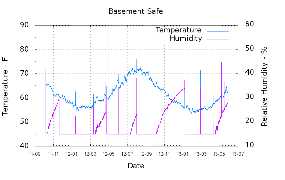
A plot of the temperature and humidity inside the basement safe over the last year-and-a-half:
Basement Safe
The tray of silica gel (or whatever those granules might be) holds the humidity firmly at 14 to 15 %, at least with a simple masking tape seal around the door opening that dates back to early 2012. Less water vapor gets through the door during the winter, due to the lower basement humidity when it’s cold outside, but it looks like four regenerations per year with just under a kilogram of desiccant in the tray.
Ordinarily, it’d be time for those granules to endure another oven session, but I just picked up a bunch of real silica gel beads and must conjure up some porous bags.
The Bash / Gnuplot script that cleaned the CSV files and produced the plot:
#!/bin/sh
#-- overhead
export GDFONTPATH="/usr/share/fonts/truetype/"
base="${1%.*}"
echo Base name: ${base}
ofile=${base}.png
tfile=$(tempfile)
echo Input file: $1
echo Temporary file: ${tfile}
echo Output file: ${ofile}
#-- prepare csv Hobo logger file
sed 's/^\"/#&/' "$1" | sed 's/^.*Logged/#&/' | sed 's/ ,/,/' | sed 's/\/\([0-9][0-9]\) /\/20\1 /' > ${tfile}
#-- do it
gnuplot << EOF
#set term x11
set term png font "arialbd.ttf" 18 size 950,600
set output "${ofile}"
set title "${base}"
set key noautotitles
unset mouse
set bmargin 4
set grid xtics ytics
set timefmt "%m/%d/%Y %H:%M:%S"
set xdata time
set xlabel "Date"
set format x "%y-%m"
#set xrange [1.8:2.2]
set xtics font "arial,12"
#set mxtics 2
#set logscale y
set ytics nomirror autofreq
set ylabel "Temperature - F"
set format y "%3.0f"
set yrange [40:90]
set mytics 2
set y2label "Relative Humidity - %"
set y2tics nomirror autofreq
set format y2 "%3.0f"
set y2range [10:60]
#set y2tics 32
#set rmargin 9
set datafile separator ","
#set label 1 "label text" at 2.100,110 right font "arialbd,18"
#set arrow from 2.100,110 to 2.105,103 lt 1 lw 2 lc 0
plot    \
    "${tfile}" using 2:3 axes x1y1 with lines lt 3 title "Temperature",\
    "${tfile}" using 2:4 axes x1y2 with lines lt 4 title "Humidity"
EOF
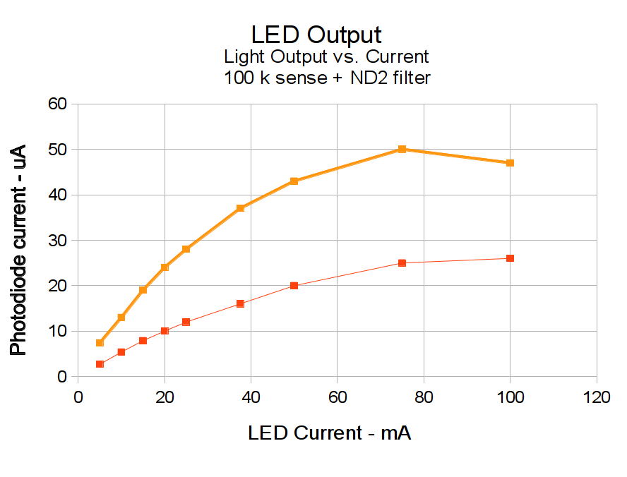
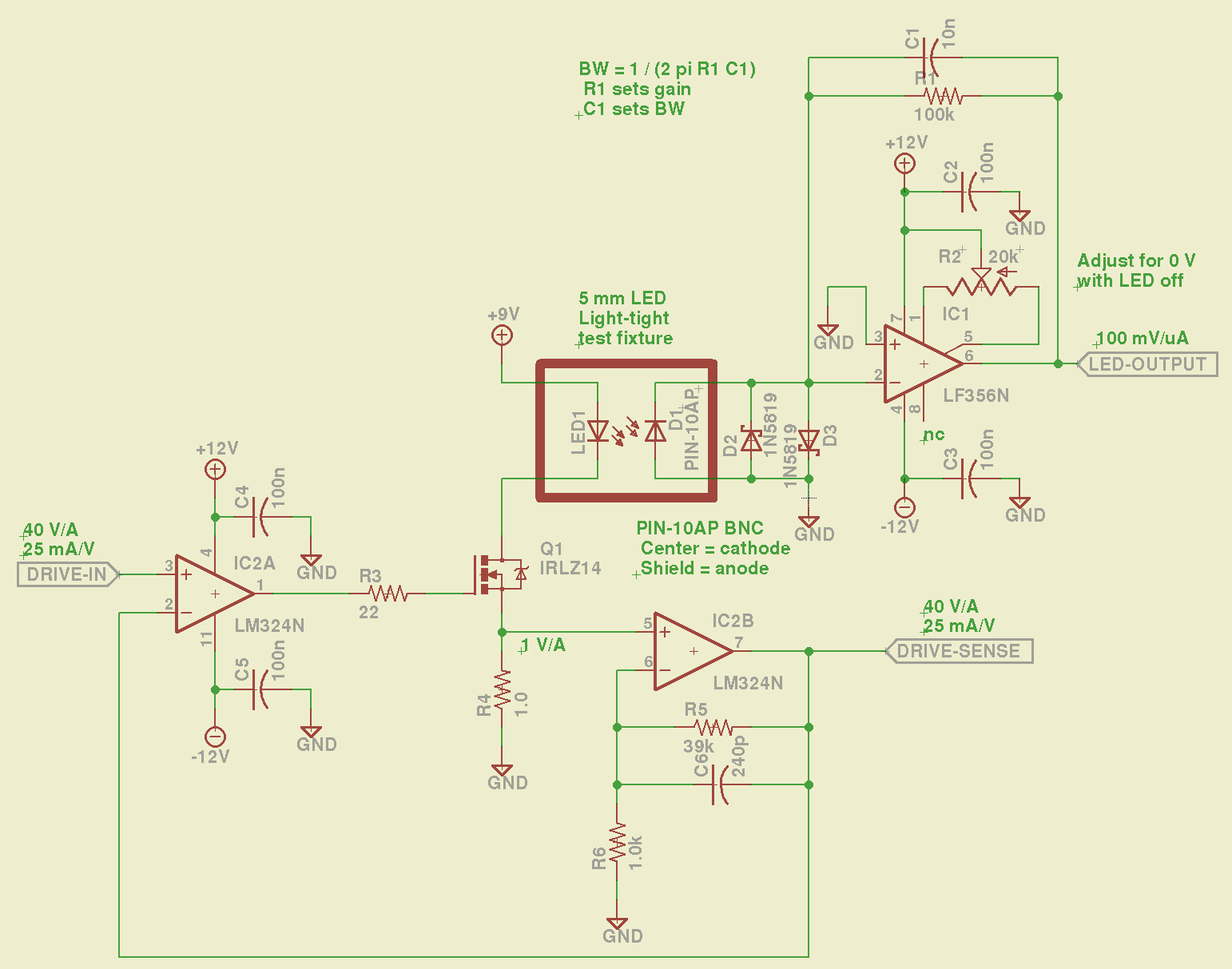
The LM324 converts the input voltage to an LED drive current, scaled by the sense resistor and the gain of IC2B to 25 mA/V. The feedback loop closes through the MOSFET and C6 rolls off the response, so there’s a nasty overshoot on the leading edge of input pulses where the current increases faster than the op amp can tamp it down:
Red LED – 25 mA 14 uA
The LM356 acts as a transimpedance amplifer to convert the photodiode current to voltage. The PIN-10AP specs say it should operate in photovoltaic mode with zero bias and that more than -3V of bias will kill the photodiode; the LM356 should hold its inverting input at virtual ground, but the two 1N5819 Schottky diodes enforce that limit. There being zero volts across the diodes, they don’t leak in either direction, so it’s all good.
The circuit is an embarrassing hairball on solderless breadboard, so use your imagination…
You could mash this together with the LED Curve Tracer, although you’d want better low-current resolution from the Arduino output.