Ed Nisley's Blog: Shop notes, electronics, firmware, machinery, 3D printing, laser cuttery, and curiosities. Contents: 100% human thinking, 0% AI slop.
Category: Science
If you measure something often enough, it becomes science
We didn’t get much more than damp and planned the ride with a bail-out route home, so it was all good.
The camera ran from STK Battery A, which had gone flat 37 minutes into a recent ride, so I popped it in the battery tester and drained the rest of its charge:
Sony NP-BX1 – STK A 27 min vs full – 2016-03-25
The dotted section says it had 0.85 W·h remaining after 27 minutes. Hand-positioning a copy of that curve against the full charge and discharge curve says the camera required 2.8 W·h. Eyeballometrically averaging the voltage over the leading part of the curve as 3.8 V says the battery delivered 0.74 A·h = 2.8 W·h / 3.8 V, then dividing that by 27/60 says the camera draws 1.6 A. That’s less than the 2 A guesstimate from previous data, but I don’t trust any of this for more than about one significant figure.
Running the camera for 27 minutes requires 2.8 W·h, meaning 37 minutes should require 3.8 W·h. The curve says that’s the capacity at the 2.8 V test cutoff, suggesting the camera also has a 2.8 V cutoff.
Looking at the discharge curves from yesterday’s post:
Sony NP-BX1 – STK ABCD – 2015-11-03 vs 2016-03-24
If all that hangs together, the C and D batteries should run the camera for just slightly longer than the A battery, but that doesn’t seem to be the actual result: they’re much better than that.
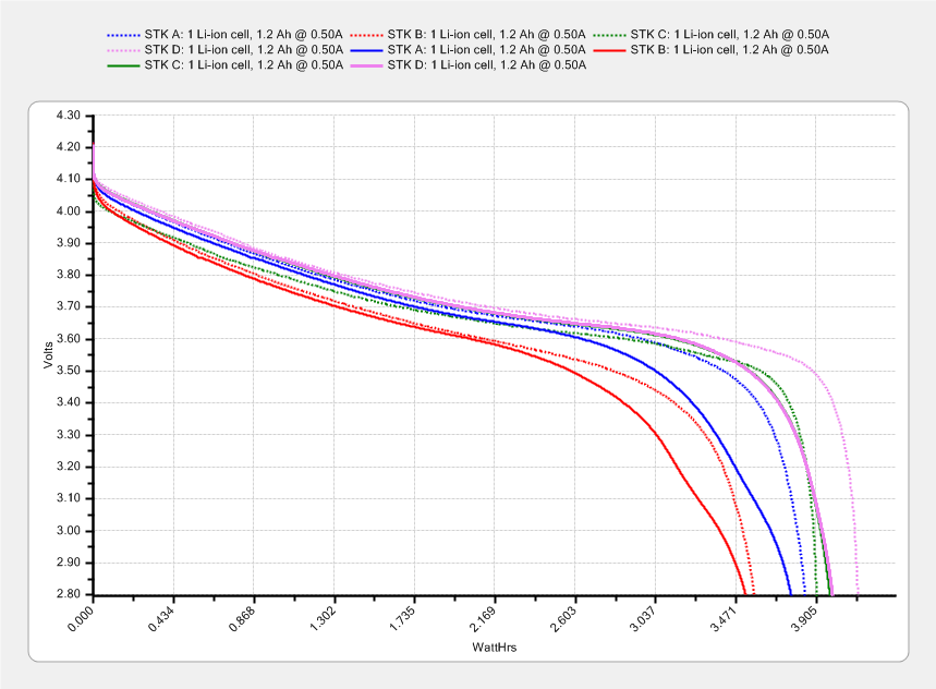
I’ve marched the four STK NP-BX1 lithium batteries through the Sony HDR-AS30V camera in constant rotation since last November. The A battery drained 35 minutes into an ordinary ride on a pleasant day, so charging and measuring the entire set seemed in order:
Sony NP-BX1 – STK ABCD – 2015-11-03 vs 2016-03-24
The dotted curves come from early November 2015, when the batteries were fresh & new, and the solid curves represent their current performance.
It’s been a mild winter, so we’ve done perhaps 75 rides during the last 150-ish days. That means each battery has experienced under 20 discharge cycles, which ought not make much difference.
The B battery started out weak and hasn’t gotten any better; I routinely change that one halfway into our longer rides.
The A battery started marginally weaker than C and D, but has definitely lost its edge: the voltage depression at the knee of the curve might account for the early shutdown.
Figuring that the camera dissipates 2.2 W, a battery that fails after 35 minutes has a capacity of 1.3 W·h. That suggests a cutoff voltage around 3.8 V, which makes absolutely no sense whatsoever, because the C and D batteries deliver at least 75 minutes = 2.8 W·h along similar voltage curves.
The B battery goes in the recycle heap and we’ll see how the A battery behaves on another ride…
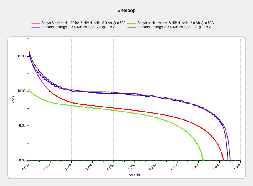
The two upper curves show the first two charges for those eight cells back in 2010.
The lower curve(s) started out with the wrong endpoint voltage (purple part of the middle curve), so I restarted the test (green curve) and edited the graph image to splice the two curves together into the purple/red curve.
Although the capacity measured in mA·h isn’t much lower, the voltage depression reduces the available energy and trips the “low battery” alarm much earlier. In round numbers, the old cells were good for a few pictures, even hot off the charger, and didn’t have much energy left without being recharged before use.
A quartet of Panasonic Eneloop Pro cells just arrived from BatterySpace, a nominally reputable supplier, all sporting a 14-05 date code suggesting they’re just shy of two years old. The packaging claims 85% charge retention after a year, so they should have a bit more than half of their rated 2.45 A·h “minimum” (or 2.55 mA·h “typical”, depending on whether you trust the label on the cell or the big print on the package) capacity remaining (although we don’t know the original state of charge, done from “solar power”). The lower curves say they arrived with 1 A·h remaining:
Panasonic Eneloop – First Charge
However, the terminal voltage on those bottom curves would have any reasonable device reporting them as dead flat almost instantly, so you really can’t store Eneloops for two years: no surprise there.
One pass through the 400 mA Sony charger produced the upper curves, with the dotted red curve from Cell A lagging in the middle. After that test, another pass through the charger brought Cell A back (upper solid red line) with the others, so I’ll assume it took a while to wake up.
A pair of these in the camera will produce 2.2 V through 2.2 A·h, far better than the aged-out Sanyo Eneloops.
Charging them at 400 mA = C/6 certainly counts as a slow charge. I’ve been charging the Sanyo cells in slow chargers in the hope that they’ll remain happier over the long term.
The fourth Sony MicroSDXC card went into service in late September 2015 and has now failed after about 60 sessions in my Sony HDR-AS30 Action Camera. This one sported a U3 speed rating and I had hopes that would improve its longevity, but that doesn’t seem to be true.
The defunct Sony card (marked in red to avoid confusion) will join its defunct compadre and the Sandisk Extreme Pro card goes in the camera:
Sony 64 GB MicroSD SR-64UX – failure
The 16 bike rides in December added up to 220 GB; call it 13.75 GB/trip. January 2016 shows only three rides and it failed after two February rides: barely 60 rides for a total of 825-ish GB of video data. The three previous Sony cards failed after less than 1 TB of data, putting this one in the same ballpark.
I have no way to measure the actual write speed, but the camera shuts down after recording less than a minute of 1920×1080 @ 60 f/s video. Previous cards worked fine at lower video resolutions and recording speeds; I’ll assume this one behaves similarly. It might make a capacious “disk” for a Raspberry Pi.
When the previous card failed, Sony’s “customer support” decided that there might be something wrong with the camera’s firmware causing it to trash the cards, so there was no point in replacing the card under warranty and I should send the camera in for a checkup. When I pointed out that they’d strung me along for a year, until the camera was out of warranty, without mentioning even the possibility that the camera might be at fault and asked whether they’d pick up the $100+ bill for having the camera “examined”, the Nice Man said Level 2 would get back to me after “48 working hours”. When prodded, he agreed that “48 working hours” equaled “6 working days” and didn’t include weekends; when we had that settled, I knew they had no further interest in this matter.
Sony hasn’t called back and, by now, I don’t expect they ever will. It’s not worth my time to pursue this any further, but if you’re wondering how well Sony MicroSD cards work in Sony cameras and how well they support the failures, now you know.
So, starting with this riding season, we’ll see how long a Sandisk Extreme Pro card survives…
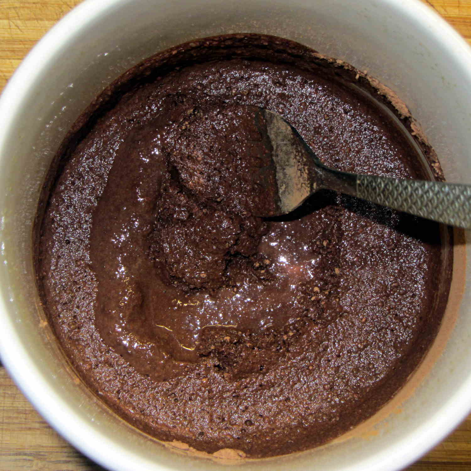
It turns out that non-alkalized / non-Dutch-process cocoa has a much lower surface energy than good old Hershey’s, to the extent that my Fireball Cocoa Recipe produces powder bombs, even after far more stirring than I’m willing to exert.
The trick is to stir the mud for a while, then let it set for 15 minutes:
Cocoa mud
That apparently gives the cocoa time to get along with the milk and join forces. Stir it up again, let it sit for a few minutes, then proceed with the recipe: smooooth cocoa with no powder bombs.
A bit more Vietmamese cinnamon is no bad thing, either …
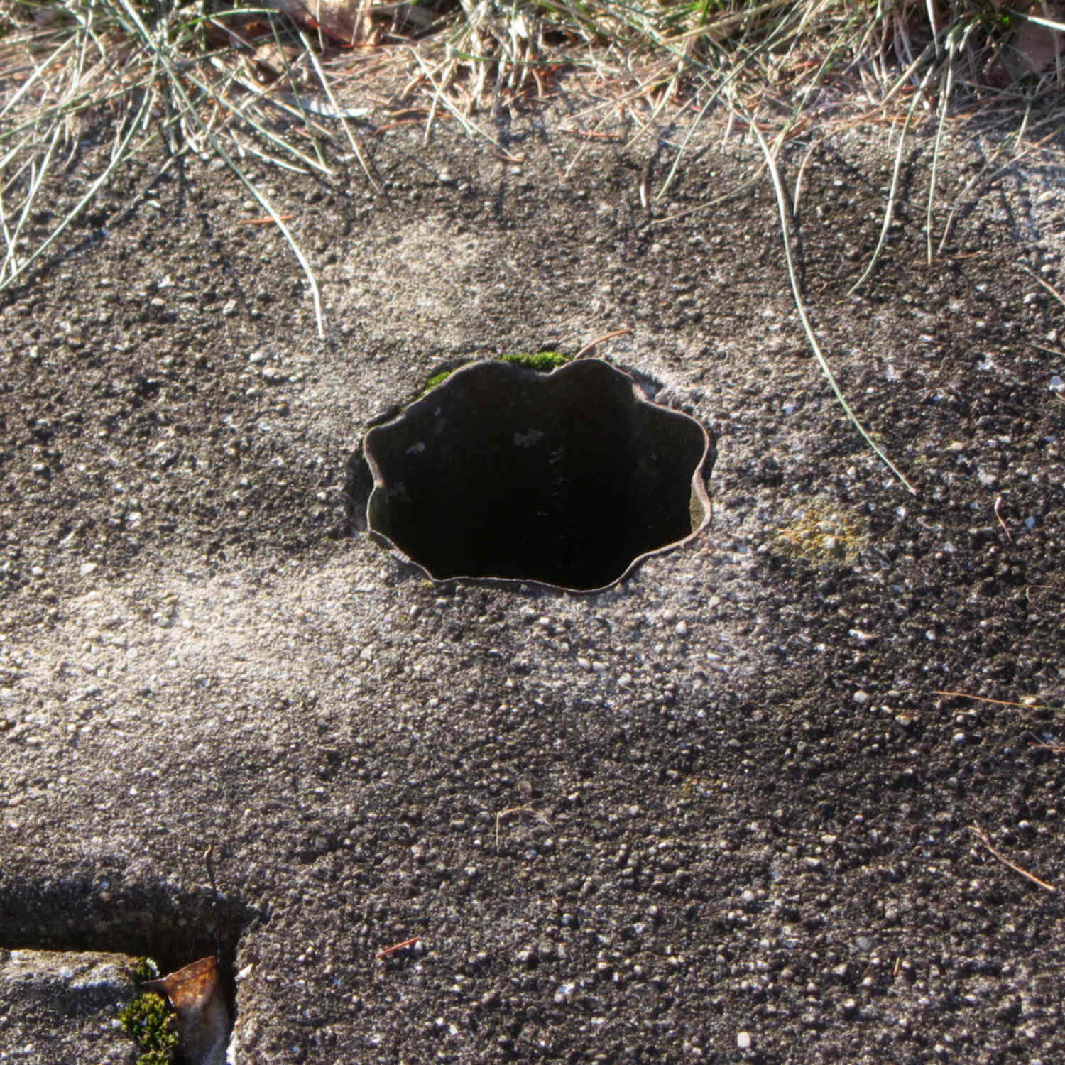
Having that knockoff Neopixel fail from overheating prompted me to measure what was going on. Because the LEDs sink most of their heat into the package leads, the back of the LED strip should be the hottest part of the package and the Mood Light’s central pillar should be pretty nearly isothermal. Despite that, I figured I should measure the temperature closer to the back of the strip, sooo I drilled a hole for the thermocouple…
Clamp the whole Mood Light to the Sherline’s tooling plate with the pillar sides mostly square to the axes and line up the spindle 2 mm behind the LED strip:
Mood Light – aligning thermocouple hole
The two clamp pads are CD chunks, under just enough pressure to anchor the Mood Light.
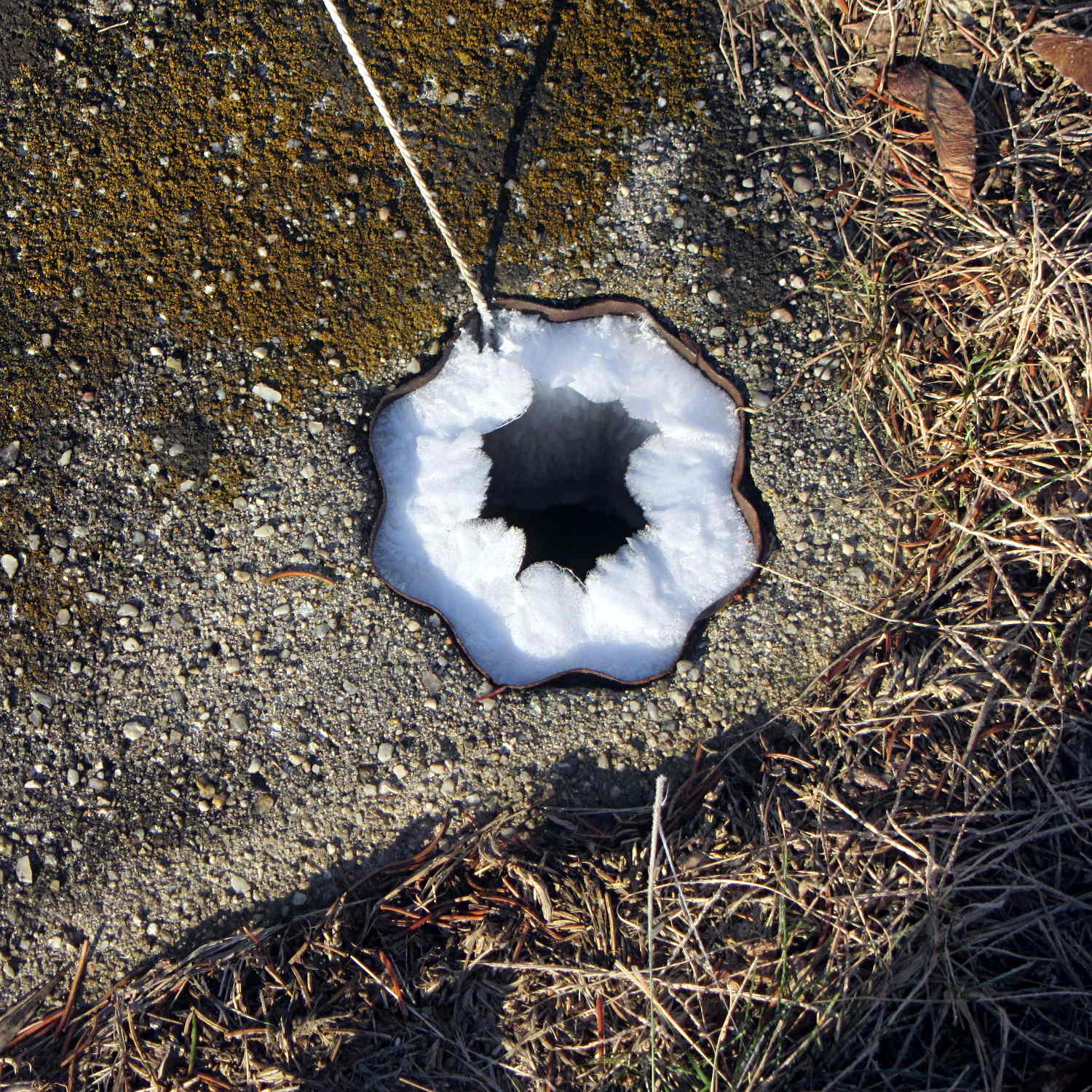
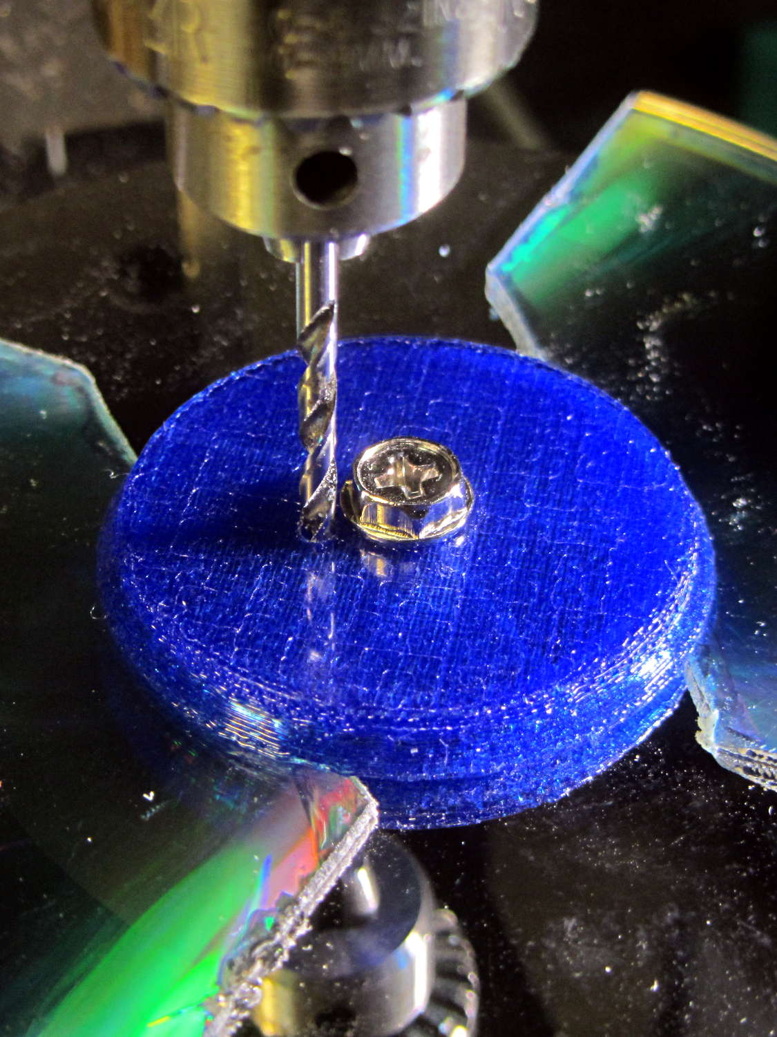
Screw the cap in place (to match-drill both holes at once) and drill a 2 mm (#46, close enough) hole down past the top LED:
Mood Light – drilling thermocouple hole
I tucked the Mood Light into a box to ward off breezes, jammed one thermocouple into the new hole, let another float over the top platter, then forced the Neopixels to display constant grayscale PWM values (R=G=B) while recording the LED and air temperatures every five minutes:
Hard Drive Mood Light – temp vs power data
That was easier and faster than screwing around with automated data collection. The data has some glaring gaps where I went off to do other things during the day.
I turned those numbers into a graph, printed it out, puzzled over it for a bit, then annotated it with useful numbers:
Hard Drive Mood Light – temp vs power data – graph
That first little blip over on the left comes from a minute or two at PWM 32; the cooling time constant works out to be a bit under 10 minutes. The warming time constant looks to be somewhat longer, but not by much.
Eyeballing the endpoint temperatures for each PWM value, feeding in the current measurements, and creating a small table:
VCC
5
V
Current
0.057
A
Package
0.285
W
Total
3.42
W
PWM
Duty
Nom Power
Failed LEDs
Net Power
°C Rise
0
0.00
0.00
0
0.00
0
32
0.13
0.43
0
0.43
6
64
0.25
0.86
0
0.86
12
85
0.33
1.14
1
1.04
16
128
0.50
1.71
1
1.62
24
192
0.75
2.57
1
2.47
35
255
1.00
3.41
4
3.03
42
The same blue LED that failed earlier dropped out again, plus another package (on a different strip) went completely dark shortly after I clobbered the LEDs with full power at PWM 255. The Net Power column deducts the power not used by the failed LEDs, under the reasonable assumption that the total heating depends on the number of active LEDs.
All the failed LEDs worked fine when they cooled to room temperature, so, whatever the failure mode might be, it’s not permanent. The skimpy WS2812B datasheet says bupkis about a protective thermal shutdown circuit, although it specs an 80 °C maximum operating junction temperature. I’ll stipulate a 20 °C temperature difference from junction to thermocouple at PWM 255, but that doesn’t explain the first blue LED failure at PWM 85.
Methinks these knockoffs will be much happier operating in the mid-30s.
Turning the last two columns of that table into a graph (minus the PWM 0 line to let the intercept float around) looks like I’m faking it:
Hard Drive Mood Light – Temperature vs Power
The Y intercept is off by less than 1 °C, which seems pretty good under the circumstances. The kink at PWM 85 shows that I probably didn’t allow enough time for the temperature to stabilize after the blue LED failed.
So, in round numbers, the thermal coefficient for a dozen knockoff Neopixels on a plastic pillar inside a stack of hard drive platters works out to 14 °C/W.
The raised sine waves in the Mood Light produce a long-term average PWM half of their maximum PWM. They’ve been perfectly happy with MaxPWM = 64 pushing them barely 6 °C over ambient, so they should continue to work fine at PWM 128 for a 12 °C rise… except, perhaps, during the hottest of mid-summer days.
Obviously, I should jam a thermistor inside the column and have the Arduino wrap a feedback loop around the column temperature…