Ed Nisley's Blog: Shop notes, electronics, firmware, machinery, 3D printing, laser cuttery, and curiosities. Contents: 100% human thinking, 0% AI slop.
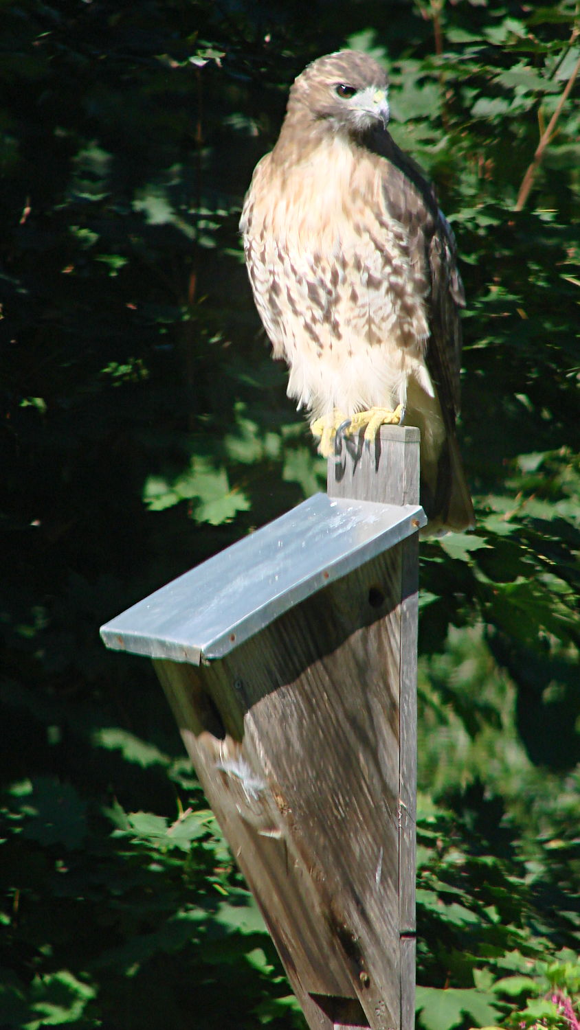
The bird box in the front lawn serves as a favorite perch for surveying the landscape:
Hawk on bird box
The chipmunks seemed fewer and farther between this summer. It’s hard to tell with chipmunks, but they seem to spend more time looking around and less time paused in the middle of the driveway.
Taken with the DSC-H5 and 1.7 teleadapter, diagonally through two layers of cruddy 1955-era window glass.
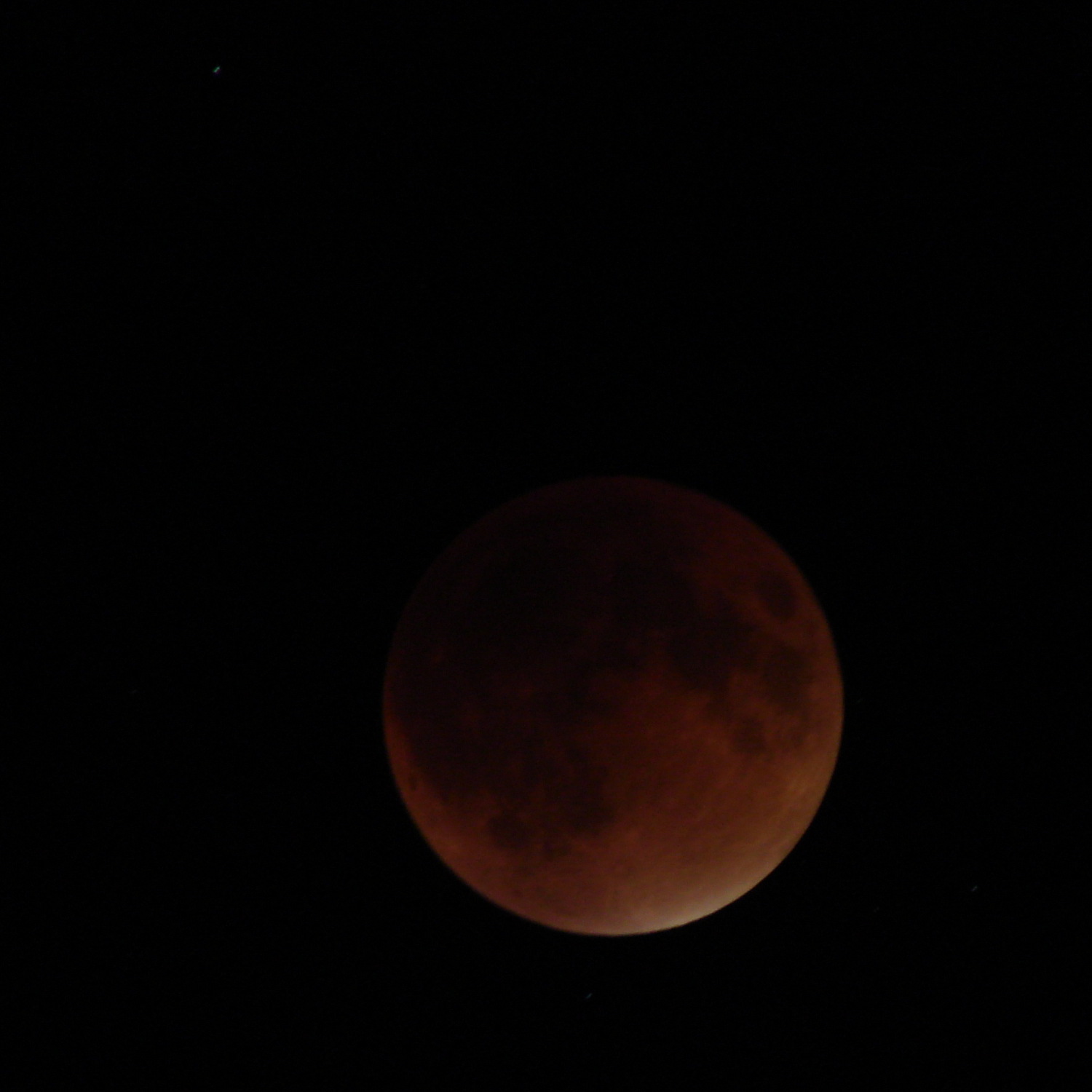
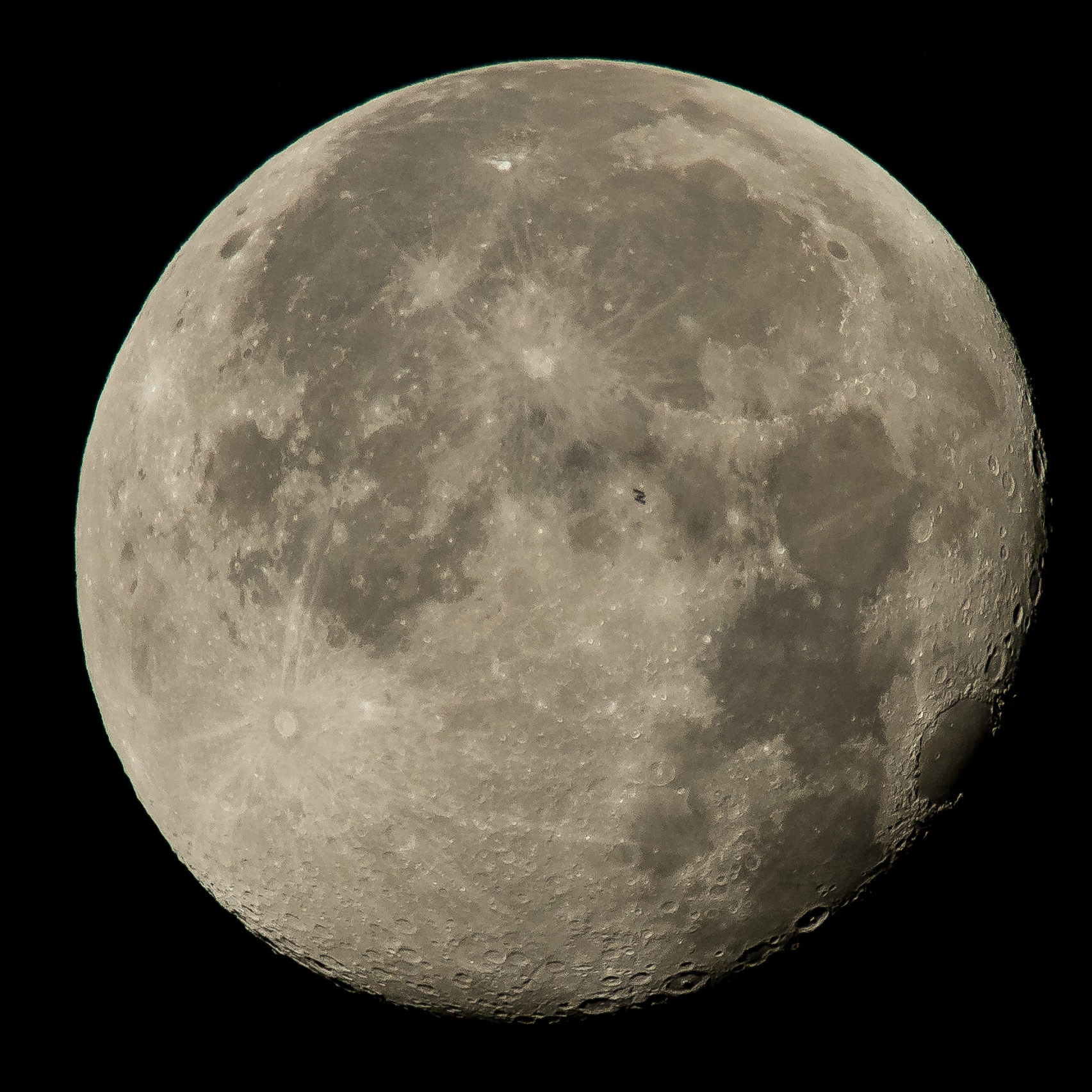
Lunar eclipses happens so rarely it’s worth going outdoors into the dark:
Supermoon eclipse 2015-09-27 2250 – ISO 125 2 s
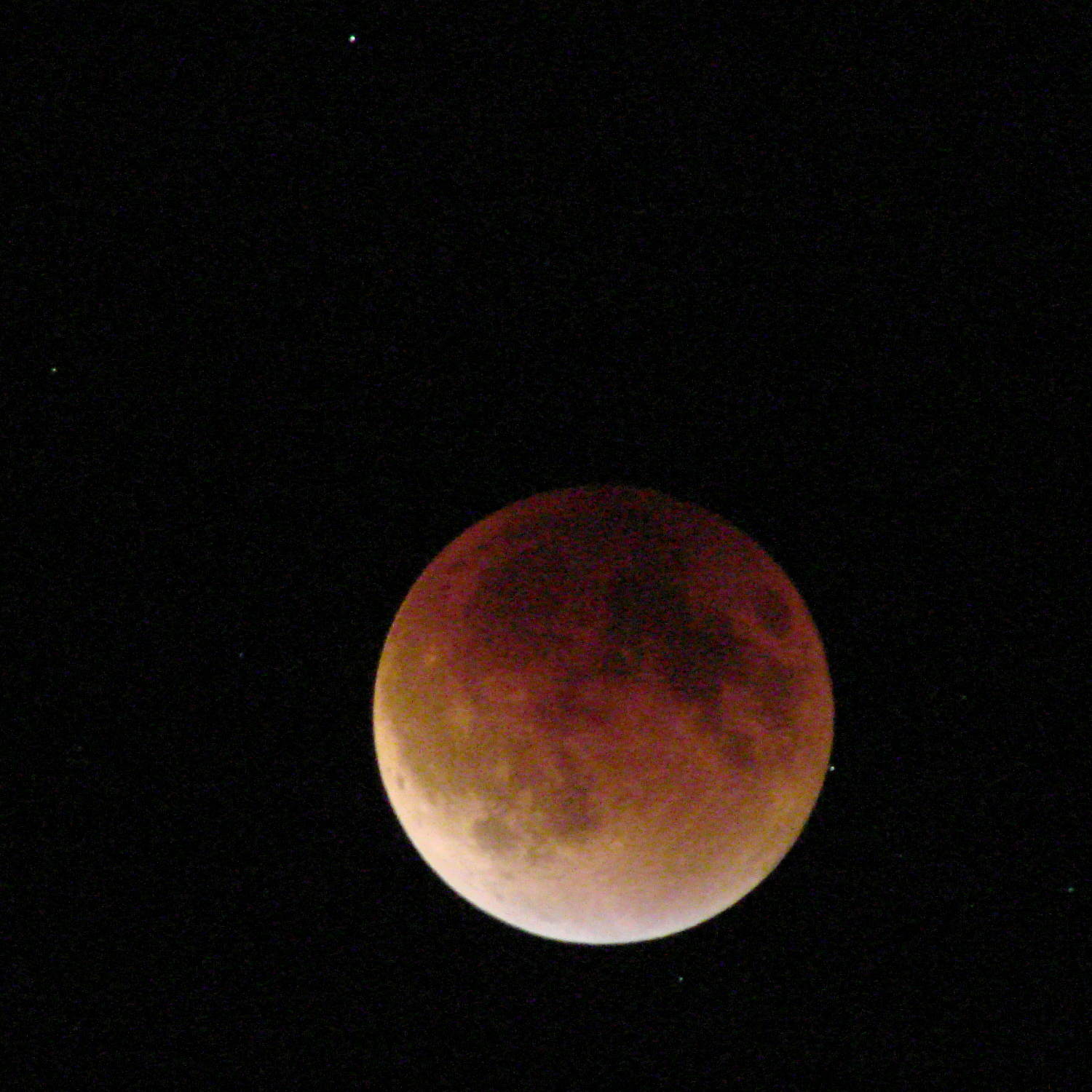
That’s at the camera’s automatic ISO 125 setting. Forcing the camera to ISO 1000 boosts the grain and brings out the stars to show just how fast the universe rotates around the earth…
One second:
Supermoon eclipse 2015-09-27 2308 – ISO 1000 1 s
Two seconds:
Supermoon eclipse 2015-09-27 2308 – ISO 1000 2 s
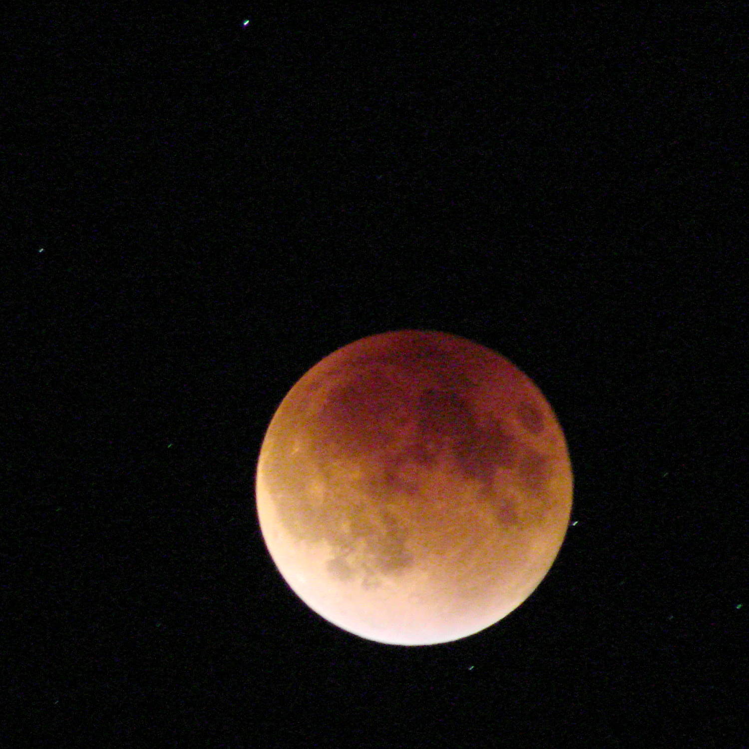
Four seconds:
Supermoon eclipse 2015-09-27 2308 – ISO 1000 4 s
Taken with the Sony DSC-H5 and the 1.7 teleadapter atop an ordinary camera tripod, full manual mode, wide open aperture at f/3.5, infinity focus, zoomed to the optical limit, 2 second shutter delay. Worked surprisingly well, all things considered.
Mad props to the folks who worked out orbital mechanics from first principles, based on observations with state-of-the-art hardware consisting of dials and pointers and small glass, in a time when religion claimed the answers and brooked no competition.
ISS Moon Transit – 2015-08-02 – NASA 19599509214_68eb2ae39f_o
The next eclipse tetrad starting in 2032 won’t be visible from North America and, alas, we surely won’t be around for the ones after that. Astronomy introduces you to deep time and deep space.
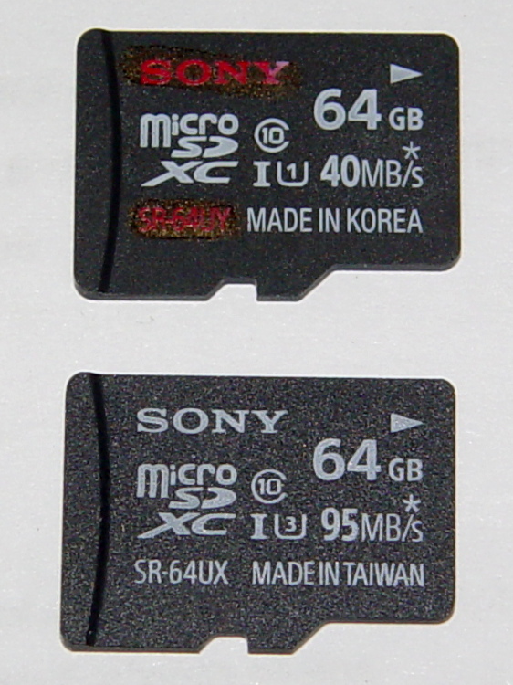
A little over a year ago, I bought two Sony 64 GB MicroSDXC cards (let’s call them A and B). Both cards failed after less than six months in service and were replaced under warranty with Cards C and D:
Sony 64 GB MicroSDXC cards – front
The top card (C) is the most recent failure, the bottom (D) is the as-yet-unused replacement for Card D. Note that the difference: SR-64UY vs. SR-64UX, the latter sporting a U3 speed rating.
Note that the failure involves the card’s recording speed, not its read-write ability or overall capacity. Card C still has its nominal 64 GB capacity and will store-and-replay data just fine, but it can’t write data at the 25 Mb/s rate required by the camera… which is barely a third of the card’s speed rating. Also note that the writing speed is always a minute fraction of the reading speed that you see on the card.
I use these in a Sony HDR-AS30V action camera on my bike, so it’s pure Sony all the way. Although I don’t keep track of every trip, I do have a pretty good idea of what happened…
In service: about 2015-07-10
Failed to record 1920×1080 @ 60 f/s video: 2015-09-22
In round numbers, that’s 70 days of regular use.
My NAS drive has room for about a month of video, depriving me of a complete record of how much data it absorbed, but from 2015-08-21 through 2015-09-22 there’s 425 GB from 25 trips in 30 days. Figuring the same intensity during the complete 70 days, it’s recorded 800 to 900 GB of data (including my verification test). With 60 GB available after formatting, that amounts to filling the card 14 times.
That’s reasonably close to the 1 TB of data I’d been estimating for the failures of Cards A and B, so these Sony cards reliably fail their speed rating after recording 750 GB, more or less, of data.
A stray sunflower seed decided that the spot just outside the garden gate was perfect and gave Mary’s garden an attractive marker. It will eventually have a dozen blossoms, each one serving as a buffet for the local bumblebees:
Sunflower with bumblebee
Each bee makes several complete circuits of the florets, draining the nectar and collecting pollen as she goes:
Sunflower with bumblebee – detail
Mary tucks the open gate inside the garden to avoid disturbing the pollinators, as wasps tend to have short fuses and multiple-strike stingers:
Sunflower with wasp
The bumblebee traveled clockwise and the wasp went counterclockwise, but I don’t know if that’s the general rule. I certainly won’t dispute their choices!
In a few weeks, long after the petals fall away, a myriad small birds will harvest the dried seeds…
Walkway Over the Hudson – Sturgeon Moonwalk – 2015-08-28
The view from the middle of the Walkway northward along the Hudson makes a nice panorama:
Walkway Over the Hudson – Sturgeon Moonwalk – North Panorama – 2015-08-28
The black rectangular lump on the left is a steel I-beam that I didn’t notice until too late.
Taken with the Canon SX-230HS, hand-braced on the rail, and stitched with The GIMP’s panorama tool. It’s surprisingly easy to stitch a decent panorama from five low-detail images with plenty of overlap…
Sticking an extruded plastic thread to the platform of a 3D printer requires absolutely accurate alignment and spacing, maybe ±0.05 mm across the entire platform. I’ll leave the topic of automatic alignment measurement & compensation for another day; here’s how to measure the actual platform alignment.
If the wall thickness (in the XY plane) doesn’t come out exactly right, fix that first by verifying the filament diameter setting, then adjusting the Extrusion Multiplier. If the extruder doesn’t produce the same wall thickness that the slicer calls for, you won’t get good results from anything else. In this case, they all have 0.40 mm thick walls, with 0.25 mm layers.
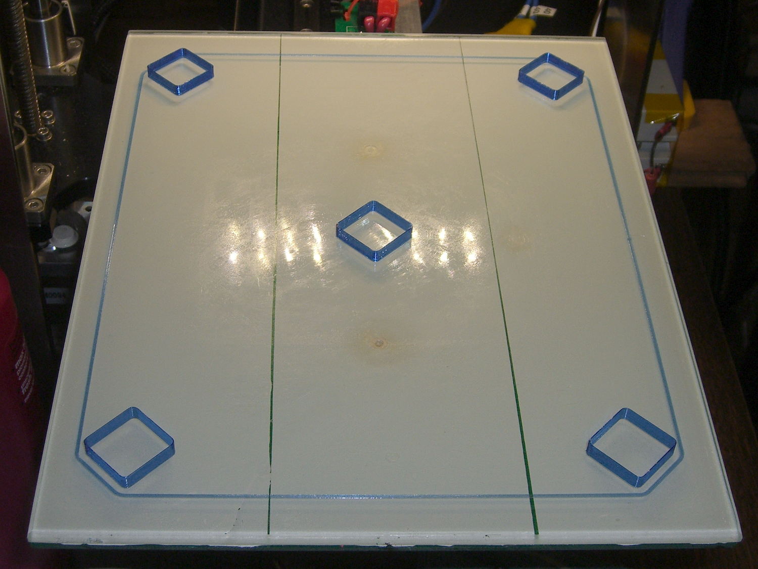
The first layer of all five boxes should be identical:
M2 V4 nozzle – thinwall box first layer
If the platform isn’t absolutely flat and properly aligned, those five first layers won’t be the same thickness. It’s surprisingly easy to spot differences under 0.05 mm, so pay attention to what’s happening.
When they’re done, pop them off and measure their actual height. I measure across adjacent sides, leaving the corners / stray hairs / snot out of the measurement, and figure the eyeballometric average of the values, which usually differ by less than ±0.03 mm. Write the height on the side to eliminate future angst:
Thinwall Box – platform height
The boxes should be 5.00 mm tall, so the leftmost box is short by -0.02 mm and the rightmost by -0.15 mm. The five boxes were 4.98, 4.95, 4.93, 4.92, and 4.85, with a mean of 4.93 mm. The variation across the 200×250 mm platform is 0.13 mm, which is pretty good.
Comparing the bottom layers of those boxes, the first layer of the 4.85 mm box is definitely squashed:
Thinwall Hollow Boxes – first layer bottom view – 4.98 4.85 mm
Once you know what to look for, it’s also obvious from the side (4.98 on the left, 4.85 on the right, bottom layers facing each other):
Thinwall boxes – 4.98 4.85 – bottom layers
Keep in mind that’s a difference of 0.13 mm = 130 µm, just over the ±0.05 mm I usually bandy about. The nominal layers are 0.25 mm = 250 µm.
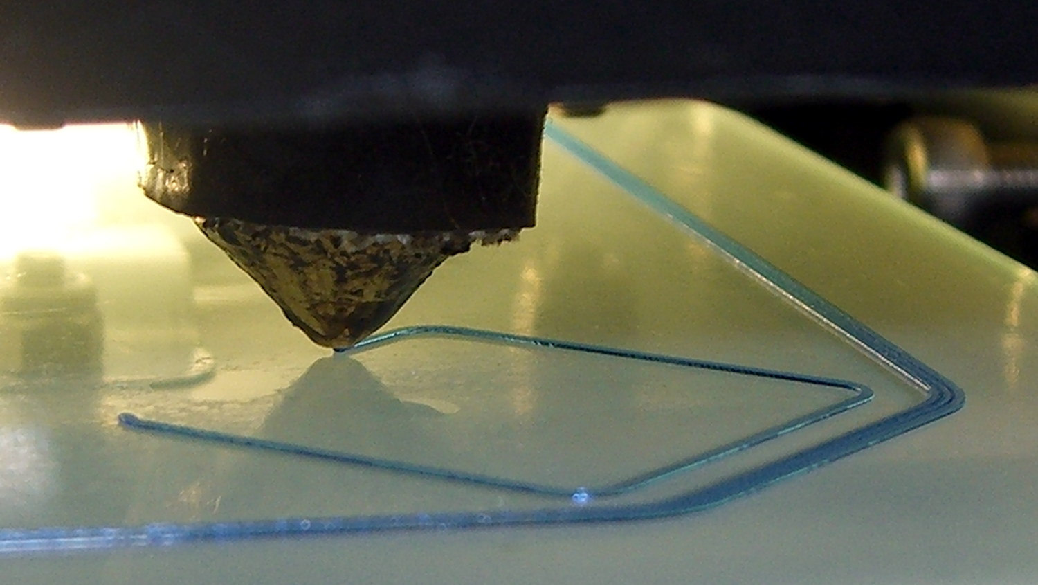
A bit more magnification shows the nicely rounded first layer of the 4.98 mm box (rightmost thread of leftmost set):
Thinwall Box – 4.98 mm
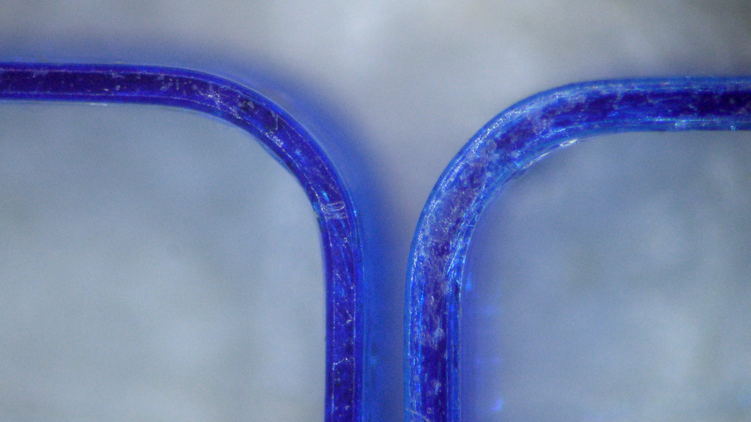
And the squashed first layer of the 4.85 mm box (likewise):
Thinwall Box – 4.85 mm
Because the Z axis moves upward (on the M2, the platform moves downward) by exactly the layer thickness at the end of each layer, the first layer must absorb the entire difference between the desired thickness and the actual nozzle-to-platform distance. That squashed first layer is 0.10 mm thick, a bit less than half of the nominal 0.25 mm. The second layer of each box looks just like all the higher layers.
You can set the Z-axis offset for a very slight squish, with the maximum nozzle-to-platform distance at 0.25 mm and the minimum set by the other end of the total misalignment, because the plastic won’t adhere to the platform when the nozzle-to-platform distance exceeds the nozzle diameter.
Think of it this way: the plastic emerges from a 0.35 mm nozzle as a (slightly larger than) 0.35 mm cylinder that must squash to become a 0.25 mm high x 0.40 mm wide thread. Given the measurements above, setting the Z-axis home position to make the average box height equal to 5.00 mm would make the tallest box come out at 5.07 mm, which requires a 0.32 mm actual first layer that probably wouldn’t stick well at all.
When your printer can consistently produce five thinwall boxes with the proper wall thickness and height, then you can move on to more complex objects.