Sticking an extruded plastic thread to the platform of a 3D printer requires absolutely accurate alignment and spacing, maybe ±0.05 mm across the entire platform. I’ll leave the topic of automatic alignment measurement & compensation for another day; here’s how to measure the actual platform alignment.
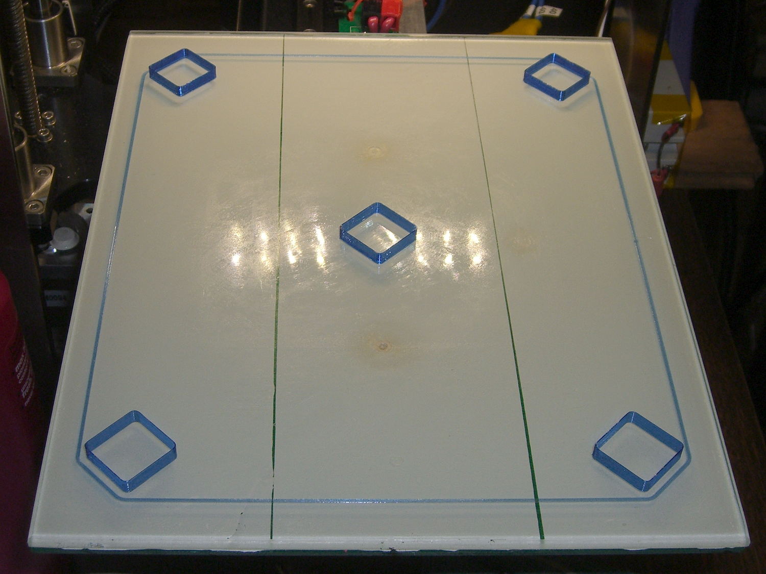
Distribute five thinwall hollow boxes across the build platform:
If the wall thickness (in the XY plane) doesn’t come out exactly right, fix that first by verifying the filament diameter setting, then adjusting the Extrusion Multiplier. If the extruder doesn’t produce the same wall thickness that the slicer calls for, you won’t get good results from anything else. In this case, they all have 0.40 mm thick walls, with 0.25 mm layers.
The first layer of all five boxes should be identical:
If the platform isn’t absolutely flat and properly aligned, those five first layers won’t be the same thickness. It’s surprisingly easy to spot differences under 0.05 mm, so pay attention to what’s happening.
When they’re done, pop them off and measure their actual height. I measure across adjacent sides, leaving the corners / stray hairs / snot out of the measurement, and figure the eyeballometric average of the values, which usually differ by less than ±0.03 mm. Write the height on the side to eliminate future angst:

The boxes should be 5.00 mm tall, so the leftmost box is short by -0.02 mm and the rightmost by -0.15 mm. The five boxes were 4.98, 4.95, 4.93, 4.92, and 4.85, with a mean of 4.93 mm. The variation across the 200×250 mm platform is 0.13 mm, which is pretty good.
Comparing the bottom layers of those boxes, the first layer of the 4.85 mm box is definitely squashed:
Once you know what to look for, it’s also obvious from the side (4.98 on the left, 4.85 on the right, bottom layers facing each other):

Keep in mind that’s a difference of 0.13 mm = 130 µm, just over the ±0.05 mm I usually bandy about. The nominal layers are 0.25 mm = 250 µm.
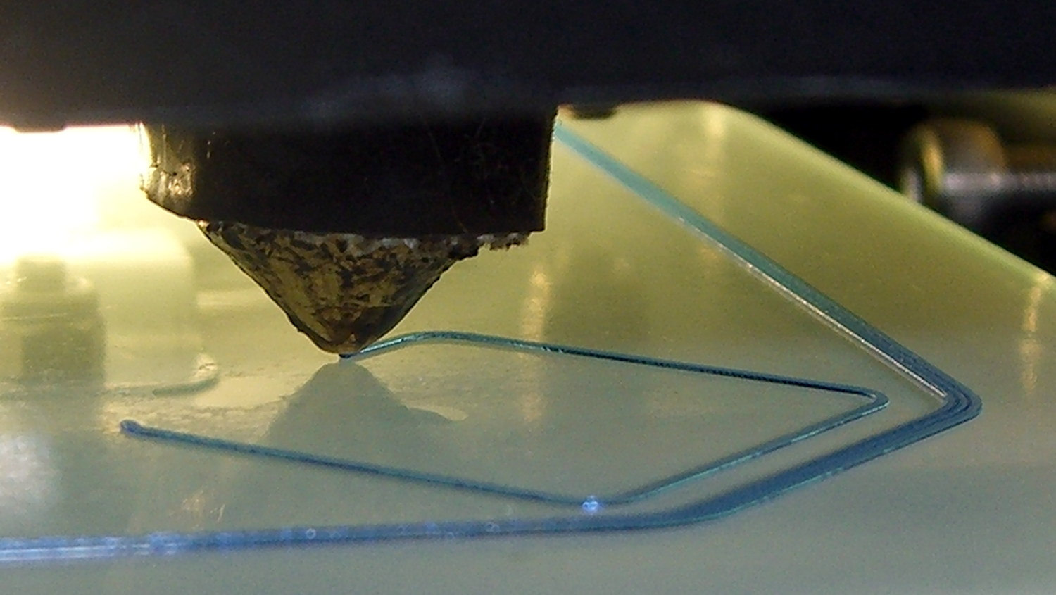
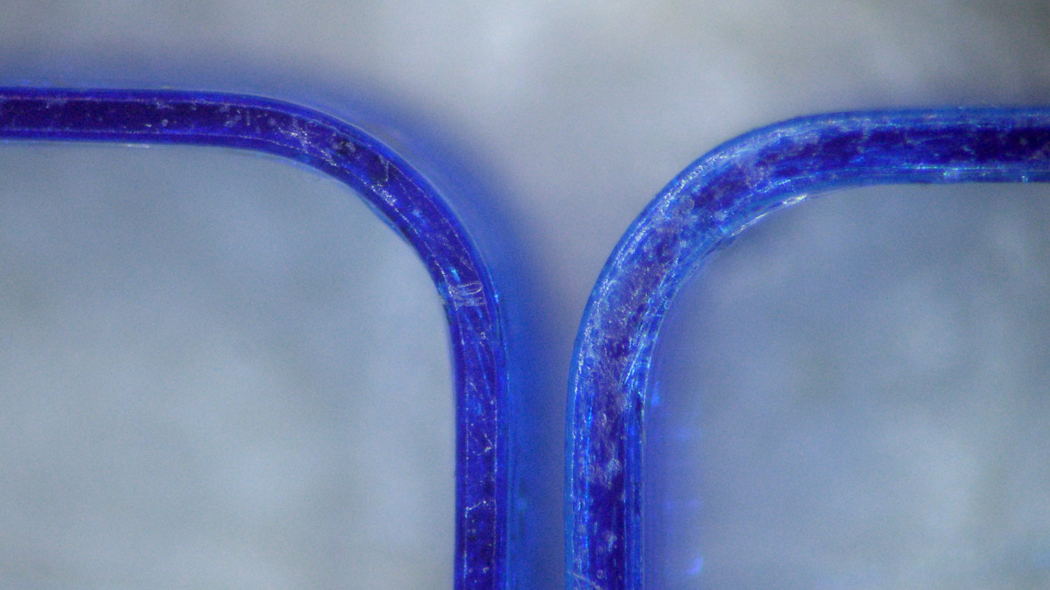
A bit more magnification shows the nicely rounded first layer of the 4.98 mm box (rightmost thread of leftmost set):

And the squashed first layer of the 4.85 mm box (likewise):

Because the Z axis moves upward (on the M2, the platform moves downward) by exactly the layer thickness at the end of each layer, the first layer must absorb the entire difference between the desired thickness and the actual nozzle-to-platform distance. That squashed first layer is 0.10 mm thick, a bit less than half of the nominal 0.25 mm. The second layer of each box looks just like all the higher layers.
Adjusting the first layer thickness by tweaking the initial Z-axis home position in the startup G-Code allows fine tuning without fussing with the mechanical settings. Having moved the Z-axis home switch to the middle of the X-axis gantry eliminates all those adjustments; tweaking the G-Code is the only way to go.
You can set the Z-axis offset for a very slight squish, with the maximum nozzle-to-platform distance at 0.25 mm and the minimum set by the other end of the total misalignment, because the plastic won’t adhere to the platform when the nozzle-to-platform distance exceeds the nozzle diameter.
Think of it this way: the plastic emerges from a 0.35 mm nozzle as a (slightly larger than) 0.35 mm cylinder that must squash to become a 0.25 mm high x 0.40 mm wide thread. Given the measurements above, setting the Z-axis home position to make the average box height equal to 5.00 mm would make the tallest box come out at 5.07 mm, which requires a 0.32 mm actual first layer that probably wouldn’t stick well at all.
When your printer can consistently produce five thinwall boxes with the proper wall thickness and height, then you can move on to more complex objects.
Selah.