Author: Ed

The original SuperFormula equation produces points in polar coordinates, which the Chiplotle library converts to the rectilinear format more useful with Cartesian plotters. I’ve been feeding the equation with 10001 angular values (10 passes around the paper, with 1000 points per pass, plus one more point to close the pattern), which means the angle changes by 3600°/10000 = 0.36° per point. Depending on the formula’s randomly chosen parameters, each successive point can move the plotter pen by almost nothing to several inches.

On the “almost nothing” end of the scale, the plotter slows to a crawl while the serial interface struggles to feed the commands. Given that you can’t see the result, why send the commands?

Computing point-to-point distances goes more easily in rectilinear coordinates, so I un-tweaked my polar-modified superformula function to return the points in rectangular coordinates. I’d originally thought a progressive scaling factor would be interesting, but it never happened.

The coordinate pruning occurs in the supershape function, which now contains a loop to scan through the incoming list of points from the  superformula function and add a point to the output path only when it differs by enough from the most recently output point:

    path = []
    path.append(Coordinate(width * points[0][0], height * points[0][1]))
    outi = 0
    xp, yp = points[outi][0], points[outi][1]
    for i in range(len(points))[1:]:
        x,y = width * points[i][0], height * points[i][1]
        dist = sqrt(pow(x - xp,2) + pow(y - yp,2))
        if dist > 60 :
          path.append(Coordinate(x, y))
          outi = i
          xp, yp = x, y

    path.append(Coordinate(width * points[-1][0], height * points[-1][1]))
    print "Pruned",len(points),"to",len(path),"points"

The first and last points always go into the output list; the latter might be duplicated, but that doesn’t matter.

Note that you can’t prune the list by comparing successive points, because then you’d jump directly from the start of a series of small motions to their end. The idea is to step through the small motions in larger units that, with a bit of luck, won’t be too ugly.

The width and height values scale the XY coordinates to fill either A or B paper sheets, with units of “Plotter Units” = 40.2 PU/mm = 1021 PU/inch. You can scale those in various ways to fit various output sizes within the sheets, but I use the defaults that fill the entire sheets with a reasonable margin. As a result, the magic number 60 specifies 60 Plotter Units; obviously, it should have a suitable name.

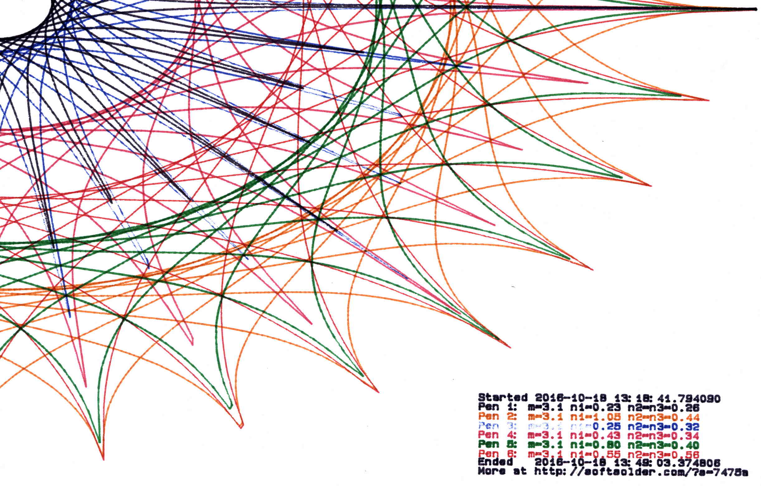
Pruning to 40 PU = 1.0 mm (clicky for more dots, festooned with over-compressed JPEG artifacts):

Pruning to 60 PU = 1.5 mm:

Pruning to 80 PU = 2.0 mm:

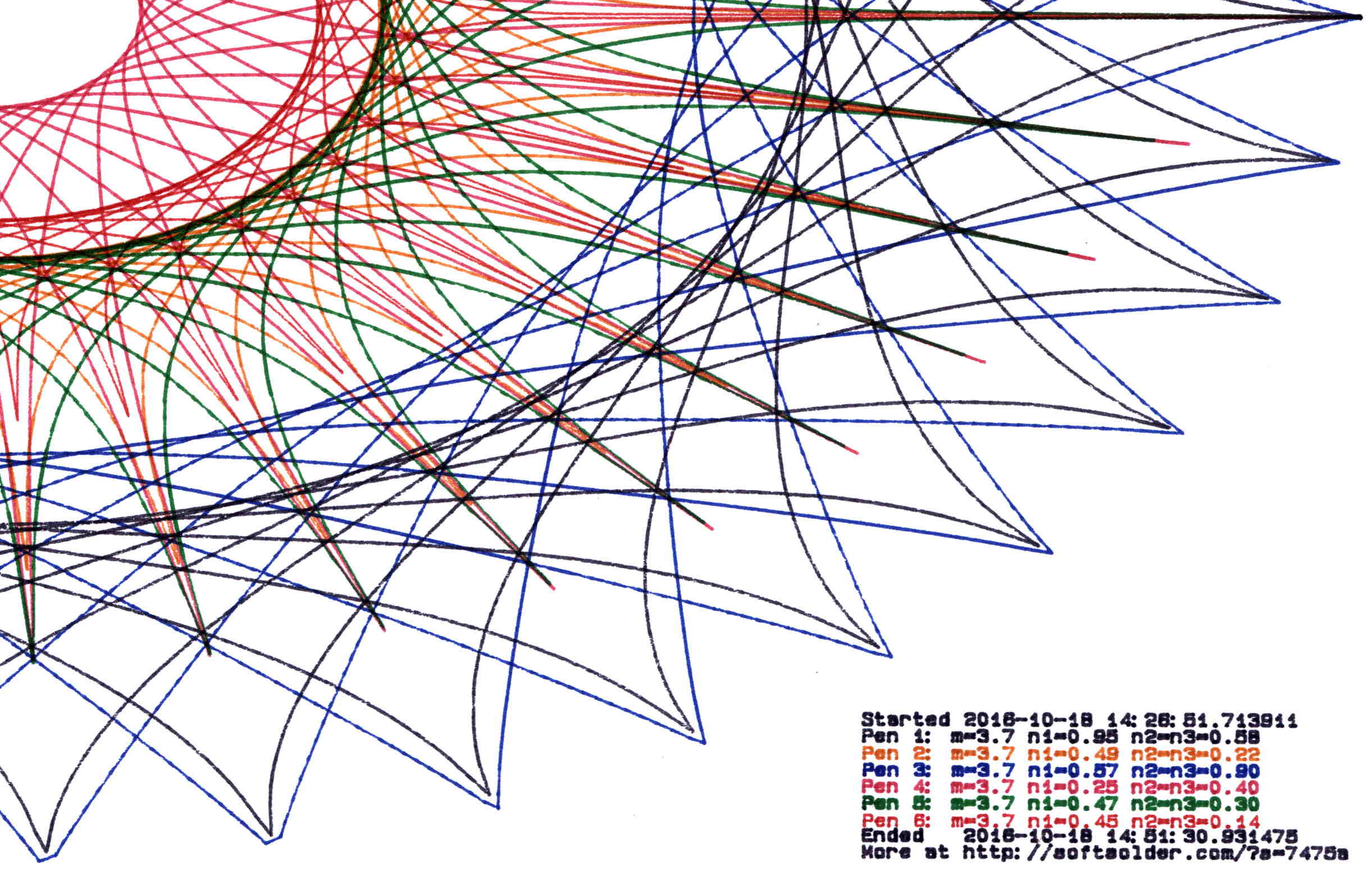
Pruning to 120 PU = 3.0 mm:

All four of those plots have the same pens in the same order, although I refilled a few of them in flight.

By and large, up through 80 PU there’s not much visual difference, although you can definitely see the 3 mm increments at 120 PU. However, the plotting time drops from just under an hour for each un-pruned plot to maybe 15 minutes with 120 PU pruning, with 60 PU producing very good results at half an hour.

Comparing the length of the input point lists to the pruned output path lists, including some pruning values not shown above:

Prune 20
1 - m: 5.3, n1: 0.15, n2=n3: 0.80
Pruned 10001 to 4856 points
2 - m: 5.3, n1: 0.23, n2=n3: 0.75
Pruned 10001 to 5545 points
3 - m: 5.3, n1: 1.15, n2=n3: 0.44
Pruned 10001 to 6218 points
4 - m: 5.3, n1: 0.41, n2=n3: 1.50
Pruned 10001 to 7669 points
5 - m: 5.3, n1: 0.29, n2=n3: 0.95
Pruned 10001 to 6636 points
6 - m: 5.3, n1: 0.95, n2=n3: 0.16
Pruned 10001 to 5076 points

Prune 40
1 - m: 3.1, n1: 0.23, n2=n3: 0.26
Pruned 10001 to 2125 points
2 - m: 3.1, n1: 1.05, n2=n3: 0.44
Pruned 10001 to 5725 points
3 - m: 3.1, n1: 0.25, n2=n3: 0.32
Pruned 10001 to 2678 points
4 - m: 3.1, n1: 0.43, n2=n3: 0.34
Pruned 10001 to 4040 points
5 - m: 3.1, n1: 0.80, n2=n3: 0.40
Pruned 10001 to 5380 points
6 - m: 3.1, n1: 0.55, n2=n3: 0.56
Pruned 10001 to 5424 points

Prune 60
1 - m: 1.1, n1: 0.45, n2=n3: 0.40
Pruned 10001 to 2663 points
2 - m: 1.1, n1: 0.41, n2=n3: 0.14
Pruned 10001 to 1706 points
3 - m: 1.1, n1: 1.20, n2=n3: 0.75
Pruned 10001 to 4446 points
4 - m: 1.1, n1: 0.33, n2=n3: 0.80
Pruned 10001 to 3036 points
5 - m: 1.1, n1: 0.90, n2=n3: 1.40
Pruned 10001 to 4723 points
6 - m: 1.1, n1: 0.61, n2=n3: 0.65
Pruned 10001 to 3601 points

Prune 80
1 - m: 3.7, n1: 0.95, n2=n3: 0.58
Pruned 10001 to 3688 points
2 - m: 3.7, n1: 0.49, n2=n3: 0.22
Pruned 10001 to 2258 points
3 - m: 3.7, n1: 0.57, n2=n3: 0.90
Pruned 10001 to 3823 points
4 - m: 3.7, n1: 0.25, n2=n3: 0.40
Pruned 10001 to 2161 points
5 - m: 3.7, n1: 0.47, n2=n3: 0.30
Pruned 10001 to 2532 points
6 - m: 3.7, n1: 0.45, n2=n3: 0.14
Pruned 10001 to 1782 points

Prune 120
1 - m: 1.9, n1: 0.33, n2=n3: 0.48
Pruned 10001 to 1561 points
2 - m: 1.9, n1: 0.51, n2=n3: 0.18
Pruned 10001 to 1328 points
3 - m: 1.9, n1: 1.80, n2=n3: 0.16
Pruned 10001 to 2328 points
4 - m: 1.9, n1: 0.21, n2=n3: 1.10
Pruned 10001 to 1981 points
5 - m: 1.9, n1: 0.63, n2=n3: 0.24
Pruned 10001 to 1664 points
6 - m: 1.9, n1: 0.45, n2=n3: 0.22
Pruned 10001 to 1290 points

Eyeballometrically, 60 PU pruning halves the number of plotted points, so the average data rate jumps from 9600 b/s to 19.2 kb/s. Zowie!

Most of the pruning occurs near the middle of the patterns, where the pen slows to a crawl. Out near the spiky rim, where the points are few & far between, there’s no pruning at all. Obviously, quantizing a generic plot to 1.5 mm would produce terrible results; in this situation, the SuperFormula produces smooth curves (apart from those spikes) that look just fine.

The Python source code as a GitHub Gist: