Ed Nisley's Blog: Shop notes, electronics, firmware, machinery, 3D printing, laser cuttery, and curiosities. Contents: 100% human thinking, 0% AI slop.
Tag: Improvements
Making the world a better place, one piece at a time
While wiring up the LED stress tester, I realized I should abuse a string of amber LEDs along with the three red strings. Herewith, four amber LEDs from the top of their bag, with LED 5 = LED 1 retested:
Amber LEDs – 100 mA
Apart from being an outlier, that red trace seems much prettier than the others, doesn’t it?
The Bash / Gnuplot routine that produced the graph has a few tweaks:
#!/bin/sh
numLEDs=4
#-- overhead
export GDFONTPATH="/usr/share/fonts/truetype/"
base="${1%.*}"
echo Base name: ${base}
ofile=${base}.png
echo Input file: $1
echo Output file: ${ofile}
#-- do it
gnuplot << EOF
#set term x11
set term png font "arialbd.ttf" 18 size 950,600
set output "${ofile}"
set title "${base}"
set key noautotitles
unset mouse
set bmargin 4
set grid xtics ytics
set xlabel "Forward Voltage - V"
set format x "%6.3f"
set xrange [1.8:2.2]
#set xtics 0,5
set mxtics 2
#set logscale y
#set ytics nomirror autofreq
set ylabel "Current - mA"
set format y "%4.0f"
set yrange [0:120]
set mytics 2
#set y2label "right side variable"
#set y2tics nomirror autofreq 2
#set format y2 "%3.0f"
#set y2range [0:200]
#set y2tics 32
#set rmargin 9
set datafile separator "\t"
set label 1 "LED 1 = LED $((numLEDs + 1))" at 2.100,110 right font "arialbd,18"
set arrow from 2.100,110 to 2.105,103 lt 1 lw 2 lc 0
plot	\
    "$1" index 0:$((numLEDs - 1)) using (\$5/1000):(\$2/1000):(column(-2)) with linespoints lw 2 lc variable,\
    "$1" index $numLEDs using (\$5/1000):(\$2/1000) with linespoints lw 2 lc 0
EOF
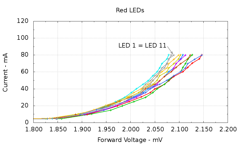
Running ten random red LEDs (taken from the bag of 100 sent halfway around the planet) through the LED Curver Tracer produces this plot:
Red LEDs – 80 mA
The two gray traces both come from LED 1 to verify that the process produces the same answer for the same LED. It does, pretty much.
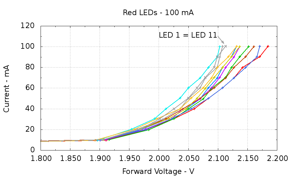
Repeating that with the same LEDs in the same order, but stepping 10 mA up to 100 mA produces a similar plot:
Red LEDs – 100 mA
The voltage quantization comes from the Arduino’s 5 mV ADC resolution (the readings are averaged, but there’s actually not much noise) and the current quantization comes from the step value in the measurement loop (5 mA in the first plot, 10 mA in the second). Seeing the LEDs line up mostly the same way at 80 mA in both graphs is comforting, as it suggests the measurement results aren’t completely random numbers.
Putting three red LEDs in series could produce a total forward drop anywhere between 6.309 V (3*2.103) and 6.555 V (3*2.185), a difference of nigh onto a quarter volt, if you assume this group spans the entire range of voltages and the whole collection has many duplicate values and you’re remarkably unlucky while picking LEDs. For this particular set, however, summing three successive groups of three produces 6.445, 6.372, and 6.469 V, for a spread of just under 100 mV. That suggests it’s probably not worthwhile to select LEDs for forward voltage within each series group of three, although matching parallel LEDs makes a lot of sense. I have no confidence the values will remain stable over power-on hours / thermal cycling / current stress.
The capacity plot for the Wouxun KG-UV3D lithium battery packs shows that there’s not a lot of capacity left after 7.0 V, so shutting down or scaling back to lower current wouldn’t be a major loss. However, it’s not clear a fixed resistor will do a sufficient job of current limiting with 6.5 V forward voltage across the LED string:
At 7.5 V, 100 mA calls for 10 Ω (drop 1 V at 100 mA)
At 8.2 V, 10 Ω produces 170 mA (1.7 V across 10 Ω)
At 7.0 V, 10 Ω produces 50 mA (0.5 V across 10 Ω)
Obviously, 170 mA is way too much, even by my lax standards.
A 100 mV variation in forward voltage between stacks, each with a 10 Ω resistor, translates into about 10 mA difference in current. This may actually call for current sensors and direct current control, although using a sensor per string, seems excessive. Low dropout regulators in current-source mode might suffice, but that still seems messy.
The test rig will run from a hard 7.5 V supply, which means I can use fixed resistors and be done with it.
The raw data behind those graphs, with LED 1 and LED 11 being the same LED:
#!/bin/sh
#-- overhead
export GDFONTPATH="/usr/share/fonts/truetype/"
base="${1%.*}"
echo Base name: ${base}
ofile=${base}.png
echo Input file: $1
echo Output file: ${ofile}
#-- do it
gnuplot << EOF
#set term x11
set term png font "arialbd.ttf" 18 size 950,600
set output "${ofile}"
set title "${base}"
set key noautotitles
unset mouse
set bmargin 4
set grid xtics ytics
set xlabel "Forward Voltage - V"
set format x "%6.3f"
set xrange [1.8:2.2]
#set xtics 0,5
set mxtics 2
#set logscale y
#set ytics nomirror autofreq
set ylabel "Current - mA"
set format y "%4.0f"
set yrange [0:120]
set mytics 2
#set y2label "right side variable"
#set y2tics nomirror autofreq 2
#set format y2 "%3.0f"
#set y2range [0:200]
#set y2tics 32
#set rmargin 9
set datafile separator "\t"
set label 1 "LED 1 = LED 11" at 2.100,110 right font "arialbd,18"
set arrow from 2.100,110 to 2.110,103 lt 1 lw 2 lc 0
plot    \
"$1" index 0:9 using (\$5/1000):(\$2/1000):(column(-2)) with linespoints lw 2 lc variable,\
"$1" index 10 using (\$5/1000):(\$2/1000) with linespoints lw 2 lc 0
EOF
And the Arduino source code, which bears a remarkable resemblance to the original firmware:
// LED Curve Tracer
// Ed Nisley - KE4ANU - December 2012

#include <stdio.h>

//----------
// Pin assignments

const byte PIN_READ_LEDSUPPLY = 0;    // AI - LED supply voltage        blue
const byte PIN_READ_VDRAIN = 1;        // AI - drain voltage            red
const byte PIN_READ_VSOURCE = 2;    // AI - source voltage            orange
const byte PIN_READ_VGATE = 3;        // AI - VGS after filtering        violet

const byte PIN_SET_VGATE = 11;        // PWM - gate voltage            brown

const byte PIN_BUTTON1 = 8;            // DI - button to start tests    green
const byte PIN_BUTTON2 = 7;            // DI - button for options        yellow

const byte PIN_HEARTBEAT = 13;        // DO - Arduino LED
const byte PIN_SYNC = 2;            // DO - scope sync output

//----------
// Constants

const int MaxCurrent = 100;                // maximum LED current - mA
const int ISTEP = 10;                    // LED current increment

const float Vcc = 4.930;                // Arduino supply -- must be measured!

const float RSense = 10.500;            // current sense resistor

const float ITolerance = 0.0005;        // current setpoint tolerance

const float VGStep = 0.019;                // increment/decrement VGate = 5 V / 256

const byte PWM_Settle = 5;                // PWM settling time ms

#define TCCRxB 0x01                        // Timer prescaler = 1:1 for 32 kHz PWM

#define MK_UL(fl,sc) ((unsigned long)((fl)*(sc)))
#define MK_U(fl,sc) ((unsigned int)((fl)*(sc)))

//----------
// Globals

float AVRef1V1;                    // 1.1 V bandgap reference - calculated from Vcc

float VccLED;                    // LED high-side supply

float VDrain;                    // MOSFET terminal voltages
float VSource;
float VGate;

unsigned int TestNum = 1;

long unsigned long MillisNow;

//-- Read AI channel
//      averages several readings to improve noise performance
//        returns value in mV assuming VCC ref voltage

#define NUM_T_SAMPLES    10

float ReadAI(byte PinNum) {

word RawAverage;

digitalWrite(PIN_SYNC,HIGH);                // scope sync

RawAverage = analogRead(PinNum);            // prime the averaging pump

for (int i=2; i <= NUM_T_SAMPLES; i++) {
RawAverage += (word)analogRead(PinNum);
}

digitalWrite(PIN_SYNC,LOW);

RawAverage /= NUM_T_SAMPLES;

return Vcc * (float)RawAverage / 1024.0;

}

//-- Set PWM output

void SetPWMVoltage(byte PinNum,float PWMVolt) {

byte PWM;

PWM = (byte)(PWMVolt / Vcc * 255.0);

analogWrite(PinNum,PWM);
delay(PWM_Settle);

}

//-- Set VGS to produce desired LED current
//        bails out if VDS drops below a sensible value

void SetLEDCurrent(float ITarget) {

float ISense;                // measured current
float VGateSet;            // output voltage setpoint
float IError;                // (actual - desired) current

VGate = ReadAI(PIN_READ_VGATE);                    // get gate voltage
VGateSet = VGate;                                    //  because input may not match output

do {

VSource = ReadAI(PIN_READ_VSOURCE);
ISense = VSource / RSense;                        // get LED current

//    printf("\r\nITarget: %lu mA",MK_UL(ITarget,1000.0));
IError = ISense - ITarget;

//    printf("\r\nISense: %d mA VGateSet: %d mV VGate %d IError %d mA",
//           MK_U(ISense,1000.0),
//           MK_U(VGateSet,1000.0),
//           MK_U(VGate,1000.0),
//           MK_U(IError,1000.0));

if (IError < -ITolerance) {
VGateSet += VGStep;
//      Serial.print('+');
}
else if (IError > ITolerance) {
VGateSet -= VGStep;
//      Serial.print('-');
}

VGateSet = constrain(VGateSet,0.0,Vcc);
SetPWMVoltage(PIN_SET_VGATE,VGateSet);

VDrain = ReadAI(PIN_READ_VDRAIN);        // sample these for the main loop
VGate = ReadAI(PIN_READ_VGATE);
VccLED = ReadAI(PIN_READ_LEDSUPPLY);

if ((VDrain - VSource) < 0.020) {            // bail if VDS gets too low
printf("# VDS=%d too low, bailing\r\n",MK_U(VDrain - VSource,1000.0));
break;
}

} while (abs(IError) > ITolerance);

//    Serial.println(" Done");
}

//-- compute actual 1.1 V bandgap reference based on known VCC = AVcc (more or less)
//        adapted from http://code.google.com/p/tinkerit/wiki/SecretVoltmeter

float ReadBandGap(void) {

word ADCBits;
float VBandGap;

ADMUX = _BV(REFS0) | _BV(MUX3) | _BV(MUX2) | _BV(MUX1);    // select 1.1 V input
delay(2); // Wait for Vref to settle

ADCSRA |= _BV(ADSC);                                        // Convert
while (bit_is_set(ADCSRA,ADSC));

ADCBits = ADCL;
ADCBits |= ADCH<<8;

VBandGap = Vcc * (float)ADCBits / 1024.0;
return VBandGap;
}

//-- Print message, wait for a given button press

void WaitButton(int Button,char *pMsg) {
printf("# %s",pMsg);
while(HIGH == digitalRead(Button)) {
delay(100);
digitalWrite(PIN_HEARTBEAT,!digitalRead(PIN_HEARTBEAT));
}

delay(50);                // wait for bounce to settle
digitalWrite(PIN_HEARTBEAT,LOW);
}

//-- Helper routine for printf()

int s_putc(char c, FILE *t) {
Serial.write(c);
}

//------------------
// Set things up

void setup() {
pinMode(PIN_HEARTBEAT,OUTPUT);
digitalWrite(PIN_HEARTBEAT,LOW);    // show we arrived

pinMode(PIN_SYNC,OUTPUT);
digitalWrite(PIN_SYNC,LOW);        // show we arrived

TCCR1B = TCCRxB;                    // set frequency for PWM 9 & 10
TCCR2B = TCCRxB;                    // set frequency for PWM 3 & 11

pinMode(PIN_SET_VGATE,OUTPUT);
analogWrite(PIN_SET_VGATE,0);        // force gate voltage = 0

pinMode(PIN_BUTTON1,INPUT_PULLUP);    // use internal pullup for buttons
pinMode(PIN_BUTTON2,INPUT_PULLUP);

Serial.begin(9600);
fdevopen(&s_putc,0);                // set up serial output for printf()

printf("# LED Curve Tracer\r\n# Ed Nisley - KE4ZNU - December 2012\r\n");

VccLED = ReadAI(PIN_READ_LEDSUPPLY);
printf("# VCC at LED: %d mV\r\n",MK_U(VccLED,1000.0));

AVRef1V1 = ReadBandGap();            // compute actual bandgap reference voltage
printf("# Bandgap reference voltage: %lu mV\r\n",MK_UL(AVRef1V1,1000.0));

}

//------------------
// Run the test loop

void loop() {

Serial.println('\n');                        // blank line for Gnuplot indexing

WaitButton(PIN_BUTTON1,"Insert LED, press button 1 to start...\r\n");
printf("# INOM\tILED\tVccLED\tVD\tVLED\tVG\tVS\tVGS\tVDS\t<--- LED %d\r\n",TestNum++);
digitalWrite(PIN_HEARTBEAT,LOW);

for (int ILED=0; ILED <= MaxCurrent; ILED+=ISTEP) {
SetLEDCurrent(((float)ILED)/1000.0);
printf("%d\t%lu\t%d\t%d\t%d\t%d\t%d\t%d\t%d\r\n",
ILED,
MK_UL(VSource / RSense,1.0e6),
MK_U(VccLED,1000.0),
MK_U(VDrain,1000.0),
MK_U(VccLED - VDrain,1000.0),
MK_U(VGate,1000.0),
MK_U(VSource,1000.0),
MK_U(VGate - VSource,1000),
MK_U(VDrain - VSource,1000.0)
);
}

SetPWMVoltage(PIN_SET_VGATE,0.0);

}
Having been unable to find a single listing of all the ARRL Hands-On Radio columns(*) by Ward Silver, N0AX, in QST magazine, I scraped their lists, did some cleanup, and roughly categorized each column’s topic. If you want to bootstrap yourself (or someone you know) from zero to pretty good, he can get you there!
[Update: (*) You must be an ARRL member to access the collection, but you need not hold an amateur radio license…]
Exp
Title
DC
Audio
Digital
Power
RF
Theory
1
The Common-Emitter Amplifier
x
x
x
x
2
The Emitter-Follower Amplifier
x
x
x
x
3
Basic Operational Amplifiers
x
x
x
4
Active Filters
x
x
5
The Integrated Timer
x
6
Rectifiers and Zener References
x
x
7
Voltage Multipliers
x
x
8
The Linear Regulator
x
x
9
Designing Drivers
x
x
x
x
10
Using SCRs
x
x
11
Comparators
x
x
x
x
12
Field Effect Transistors
x
x
x
x
x
x
13
Attenuators
x
x
x
14
Optocouplers
x
x
x
15
Switchmode Regulators, Part 1
x
x
16
Switchmode Regulators, Part 2
x
x
17
The Phase-Shift Oscillator
x
x
x
18
Frequency Response
x
x
x
19
Current Sources
x
x
x
20
The Differential Amplifier
x
x
21
The L-Network
x
x
22
Stubs
x
x
23
Open House in the N0AX Lab
24
Heat Management
x
x
25
Totem Pole Outputs
x
x
x
x
26
Solid-State RF Switches
x
27
Scope Tricks
x
x
x
x
x
x
28
The Common Base Amplifier
x
x
x
x
29
Kirchhoff’s Laws
x
x
x
30
The Charge Pump
x
x
x
x
31
The Multivibrator
x
x
x
32
Thevenin Equivalents
x
33
The Transformer
x
x
x
x
34
Technical References
x
35
Power Supply Analysis
x
x
x
36
The Up-Down Counter
x
37
Decoding for Display
x
38
Battery Charger
x
x
39
Battery Charger, Part 2
x
x
40
VOX
x
41
Damping Factor
x
x
x
42
Notch Filters
x
x
x
43
RF Oscillators, Part 1
x
x
44
RF Oscillators, Part 2
x
x
45
RF Amplifiers, Part 1
x
x
x
46
Two Cs: Crystal and Class
x
x
47
Toroids
x
x
48
Baluns
x
x
49
Reading and Drawing Schematics
x
50
Filter Design 1
x
x
x
51
Filter Design 2
x
x
x
52
SWR Meters
x
53
RF Peak Detector
x
x
x
54
Precision Rectifiers
x
x
55
Current/Voltage Converters
x
x
x
x
56
Design Sensitivities
x
57
Double Stubs
x
58
Double Stubs II
x
59
Smith Chart Fun I
x
x
60
Smith Chart Fun 2
x
x
61
Smith Chart Fun 3
x
x
62
About Resistors
x
x
x
x
63
About Capacitors
x
x
x
x
64
Waveforms and Harmonics
x
x
x
x
x
65
Spectrum Modification
x
x
x
66
Mixer Basics
x
x
x
x
67
The Return of the Kit
68
Phase Locked Loops, the Basics
x
x
x
x
69
Phase Locked Loops, Applications
x
x
x
70
Three-Terminal Regulators
x
x
x
71
Circuit Layout
x
x
x
x
x
x
72
Return Loss and S-Parameters
x
x
73
Choosing an Op Amp
x
x
x
74
Resonant Circuits
x
x
x
75
Series to Parallel Conversion
x
x
76
Diode Junctions
x
x
x
77
Load Lines
x
x
x
x
78
Bridge Circuits
x
x
x
79
Pi and T Networks
x
x
x
80
Battery Capacity
x
x
x
81
Synchronous Transformers
x
x
82
Antenna Height
x
x
83
Circuit Simulation, Part One
x
x
x
x
x
x
83
Circuit Simulation, Build and Test
x
x
x
x
x
x
85
Circuit Simulation, Complex Parts
x
x
x
x
x
x
86
Viewing Waveforms in LTspice
x
x
x
x
x
87
Elsie Filter Design, Part 1
x
x
88
Elsie Filter Design, Part 2
x
x
89
Overvoltage Protection
x
x
x
x
90
Construction Techniques
x
x
x
x
91
Common Mode Choke
x
x
x
92
The 468 Factor
x
x
93
An LED AM Modulator
x
94
SWR and Transmission Line Loss
x
x
95
Watt’s In a Waveform?
x
x
x
x
x
96
Open Wire Transmission Lines
x
97
Programmable Frequency Reference
x
x
x
98
Linear Supply Design
x
x
x
99
Cascode Amplifier
x
x
x
x
100
Hands-On Hundred
101
Rotary Encoders
x
102
Detecting RF, Part 1
x
x
x
x
103
Detecting RF, Part 2
x
x
x
x
104
Words to Watch For
x
105
Gain-Bandwidth Product
x
x
x
x
106
Effects of Gain-Bandwidth Product
x
x
x
107
PCB Layout, Part 1
x
x
x
x
x
x
108
PCB Layout, Part 2
x
x
x
x
x
x
109
PCB Layout, Part 3
x
x
x
x
x
x
110
PCB Layout, Part 4
x
x
x
x
x
x
111
Coiled-Coax Chokes
x
112
RFI Hunt
x
x
113
Radiation Patterns
x
x
114
Recording Signals
x
x
115
All About Tapers
x
x
116
The Quarter-Three-Quarter Wave Balun
x
117
Laying Down the Laws
x
118
The Laws at Work
x
119
The Q3Q Balun Redux
x
120
Power Polarity Protection
x
x
Corrections, amendations, commentary? Let me know…
The tech reviewer for my Circuit Cellar columns on the MOSFET tester commented that the 32 kHz PWM frequency I used for the Peltier module temperature controller was much too high:
Peltier Noise – VDS – PWM Shutdown
He thought something around 1 Hz would be more appropriate.
Turns out we were both off by a bit. That reference suggests a PWM frequency in the 300-to-3000 Hz range. The lower limit avoids thermal cycling effects (the module’s thermal time constant is much slower) and, I presume, the higher limit avoids major losses from un-snubbed transients (they still occur, but with a very low duty cycle).
Peltier Turn-Off Transient
The Peltier PWM drive comes from PWM 10, which uses Timer 1. The VDS and ID setpoints come from PWM 11 and PWM 3, respectively, which use Timer 2. So I can just not tweak the Timer 1 PWM frequency, take the default 488 Hz, and it’s all good. That ever-popular post has the frequency-changing details.
Although it’s common practice to exchange your empty 20 pound propane tank for a full one, I vastly prefer to keep my own tanks: I know where they’ve been, how they’ve been used, and can be reasonably sure they don’t have hidden damage. Two of my tanks have old-style threaded connections, but the barby has a quick-disconnect fitting on the regulator and I’ve been using an adapter on those tanks.
The adapter comes with a plastic tool that you use to install it in the tank valve. In principle, you insert the tool into the adapter, thread the adapter into the valve, then tighten with a wrench until the neck of the plastic tool snaps, at which point you eject the stub and the adapter becomes permanently installed. I don’t like permanent, so I carefully tightened the adapter to the point where the O-ring seals properly and the tool didn’t quite break. I’ve always wanted a backup tool, just in case the original broke, and now I have one:
Propane QD Adapter Tool – in adapter
It fit into both the adapter body and the 5/8 inch wrench (the OEM tool is 9/16 inch) without any fuss at all:
Propane QD Adapters – OEM and printed
The solid model has a few improvements over the as-printed tool above:
Shorter wrench flats
More durable protrusions to engage the locking balls
Propane QD Adapter Tool
It took about an hour to design and another 45 minutes to print, so it’s obviously not cost-effective. I’ll likely never print another, but maybe you will.
The OpenSCAD source code:
// Propane tank QD connector adapter tool
// Ed Nisley KE4ZNU November 2012

include </mnt/bulkdata/Project Files/Thing-O-Matic/MCAD/units.scad>
include </mnt/bulkdata/Project Files/Thing-O-Matic/Useful Sizes.scad>

//- Extrusion parameters must match reality!
//  Print with +1 shells and 3 solid layers

ThreadThick = 0.25;
ThreadWidth = 2.0 * ThreadThick;

HoleWindage = 0.2;

function IntegerMultiple(Size,Unit) = Unit * ceil(Size / Unit);

Protrusion = 0.1;			// make holes end cleanly

//----------------------
// Dimensions

WrenchSize = (5/8) * inch;		// across the flats
WrenchThick = 10;

NoseDia = 8.6;
NoseLength = 9.0;

LockDia = 12.5;
LockRingLength = 1.0;
LockTaperLength = 1.5;

TriDia = 15.1;
TriWide = 12.2;										// from OD across center to triangle side
TriOffset = TriWide - TriDia/2;		// from center to triangle side
TriLength = 9.8;

NeckDia = TriDia;
NeckLength = 4.0;

//----------------------
// Useful routines

module PolyCyl(Dia,Height,ForceSides=0) {			// based on nophead's polyholes

Sides = (ForceSides != 0) ? ForceSides : (ceil(Dia) + 2);

FixDia = Dia / cos(180/Sides);

cylinder(r=(FixDia + HoleWindage)/2,
h=Height,
	   $fn=Sides);
}

module ShowPegGrid(Space = 10.0,Size = 1.0) {

Range = floor(50 / Space);

	for (x=[-Range:Range])
	  for (y=[-Range:Range])
		translate([x*Space,y*Space,Size/2])
		  %cube(Size,center=true);

}

//-------------------
// Build it...

$fn = 4*6;

ShowPegGrid();

union() {

	translate([0,0,(WrenchThick + NeckLength + TriLength - LockTaperLength - LockRingLength + Protrusion)])
		cylinder(r1=NoseDia/2,r2=LockDia/2,h=LockTaperLength);

		translate([0,0,(WrenchThick + NeckLength + TriLength - LockRingLength)])
		cylinder(r=LockDia/2,h=LockRingLength);

	difference() {
		union() {

			translate([0,0,WrenchThick/2])
				cube([WrenchSize,WrenchSize,WrenchThick],center=true);

			cylinder(r=TriDia/2,h=(WrenchThick + NeckLength +TriLength));

			cylinder(r=NoseDia/2,h=(WrenchThick + NeckLength + TriLength + NoseLength));
		}

		for (a=[-1:1]) {
			rotate(a*120)
				translate([(TriOffset + WrenchSize/2),0,(WrenchThick + NeckLength + TriLength/2 + Protrusion/2)])
					cube([WrenchSize,WrenchSize,(TriLength + Protrusion)],center=true);
		}
	}
}
After 30 years, IBM gave Mary a commemorative clock, after which she promptly retired. Back in the day, they used to hand out Atmos clocks (admittedly, on more momentous occasions), but this isn’t one of those. In fact, although it appears to have a torsion pendulum, that’s a separate motor-driven foo-foo which we immediately turned off:
Janus Clock – front
It normally sits on the living room coffee table (which actually holds a myriad plants next to the front window) where, after we scrapped all the upholstered furniture, the two of us can’t both see the clock face from our chairs. Having a spare clock insert from that repair, we had the same bright idea at the same time: we need a clock with two faces! We came up with Janus independently…
Despite its fancy appearance, the IBM clock consists mostly of brass and plastic, so I had no qualms about having my way with it in the shop. The new clock insert spanned the clock’s gilt plastic back cover, needing only a #1 drill hole for the adjustment stem, and exactly filled the available space between the back cover and the case. Both movements had enough interior clearance for 3-48 brass screw heads and nuts, so I eyeballed the right spots on the new cover, centered the Sherline spindle on the plate, and drilled two clearance holes 6 mm in from the edges on the vertical diameter:
Drilling clock insert cover
That put them 61.3 mm apart across the diameter, which would be awkward to duplicate by hand. Manual CNC makes it trivially easy to match-drill holes; I clamped down the gilt back cover from the IBM clock, aligned it to the table, located the center, and drilled two 3-48 clearance holes:
Drilling torsion clock cover
The glow from that polycarbonate packing block isn’t quite so nuclear in real life. The clamping force goes down the side panels of the cover, which had enough of a curve to be perfectly stable. Yes, I’m drilling into air, but came down real slow using the Joggy Thing and it was all good.
Assemble the two back covers (the holes matched perfectly), mark the adjustment stem hole, disassemble, hand-drill, reassemble, tighten nuts, and install:
Janus Clock – rear
It does look a bit lumpy from the side, but that’s just because I don’t have any gilding for the black tape wrap: