Ed Nisley's Blog: Shop notes, electronics, firmware, machinery, 3D printing, laser cuttery, and curiosities. Contents: 100% human thinking, 0% AI slop.
A bag of 50 cheap Hall effect sensors arrived from the usual eBay vendor, who was different from all previous eBay vendors (if in name only). Passing 124 mA through the armored FT50 toroid with 25 turns of 26 AWG wire, we find this distribution of bias points, measured as the offset from the actual VCC/2:
eBay 49E Hall Effect Sensor Bias Histogram
The bias point is actually referenced to the negative terminal (usually ground) with a ±0.25 V variation around the nominal. SS49 sensors run about 0.5 V below VCC/2 (2.25 V with a 5 V supply), SS49E sensors at 2.5 V with a tighter VCC limit that suggests you better stay pretty close to 5.0 V.
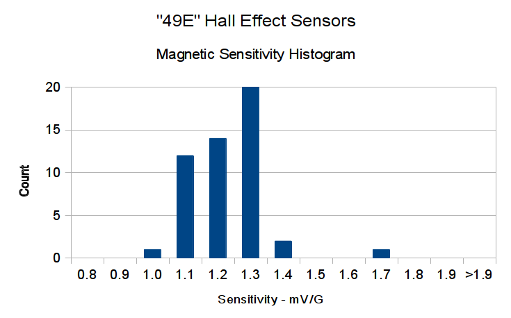
Allowing for the fact that I really don’t have good control over the actual magnetic field, the gain distribution seems tight:
eBay 49E Hall Effect Sensor Sensitivity Histogram
You’ll recall the Genuine Honeywell sensor specs:
SS49 – nominal 0.9 mV/G, limits 0.6 to 1.25 mV/G
SS49E – nominal 1.4 mV/G, limits 1.0 to 1.75 mV/G
The gain is roughly half that of the previous “49E” sensors, confirmed by sticking one of them this field. I don’t know which is more accurate, but these have a much prettier distribution.
So this lot resembles 49E sensors in both bias and gain.
Given the bias variation, though, it’s obvious that a DC application must measure the zero-field output and apply an analog offset to the amplifier, because a twiddlepot setting won’t suffice. Most likely, you’d want to update the offset every now and again to compensate for temperature variation, too.
Tossing the outliers gives an average gain of 1.17, which would give results within 10% over the lot. Given that you don’t care about the actual magnetic field, you could calibrate the output voltage for a known input current and get really nice results.
If you were doing position sensing from a known magnet, you’d want better control of the magnetic field gradient.
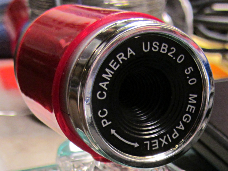
A brace of “Fashion” USB video cameras arrived from halfway around the planet. According to the eBay description and the legend around the lens, they’re “5.0 Megapixel”:
Fashion USB camera – case front
The reality, of course, is that for five bucks delivered you get 640×480 VGA resolution at the hardware level and their Windows driver interpolates the other 4.7 megapixels. VGA resolution will be good enough for my simple needs, particularly because the lens has a mechanical focus adjustment; the double-headed arrow symbolizes the focus action.
But the case seemed entirely too bulky and awkward. A few minutes with a #0 Philips screwdriver extracted the actual camera hardware, which turns out to be a double-sided PCB with a lens assembly on the front:
Fashion USB video – case vs camera
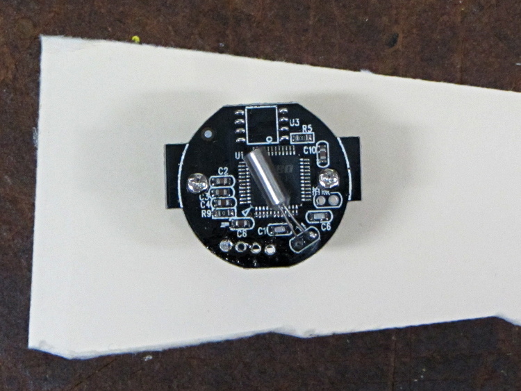
The PCB has asymmetric tabs that ensure correct orientation in the case:
Fashion USB camera – wired PCB rear
In order to build an OpenSCAD model for a more compact case, we need the dimensions of that PCB and those tabs…
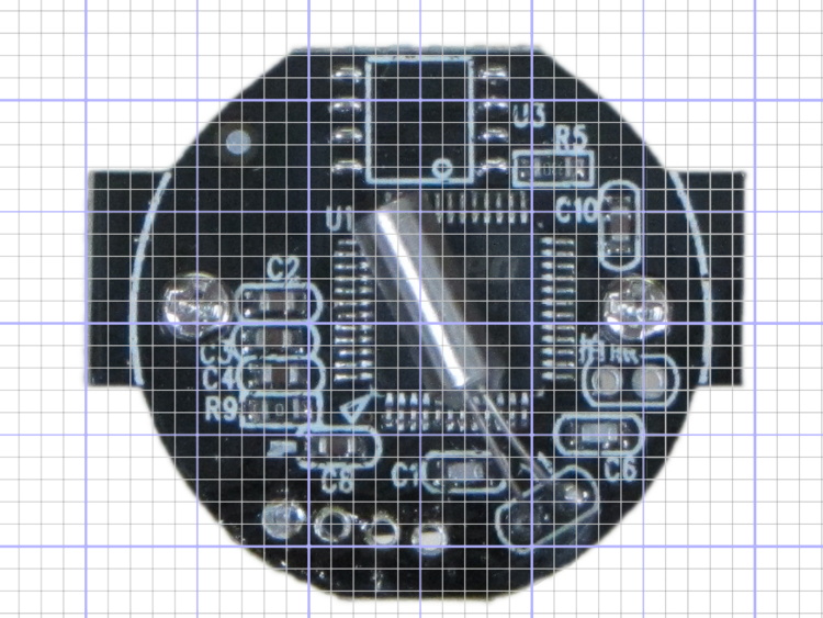
Start with a picture of the back of the PCB against white paper, taken from a few feet to flatten the perspective:
img_3300 – Camera PCB on white paper
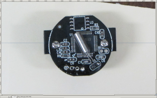
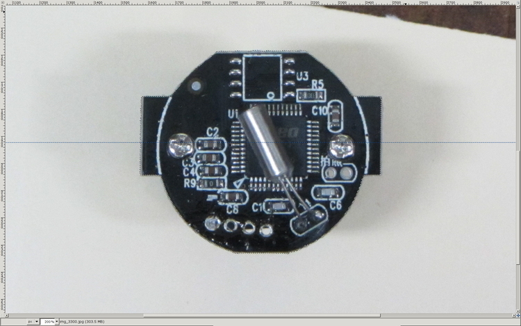
Load it into The GIMP, zoom in, and pull a horizontal guide line down to about the middle of the image:
Camera PCB – horizontal guide – scaled
Rotate to align the two screws horizontally (they need not be centered on the guide, just lined up horizontally):
Camera PCB – rotated to match horizontal guide – scaled
Use the Magic Scissors to select the PCB border (it’s the nearly invisible ragged dotted outline):
Camera PCB – scissors selection – scaled
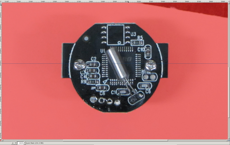
Flip to Quick Mask mode and clean up the selection as needed:
Camera PCB – quick mask cleanup – scaled
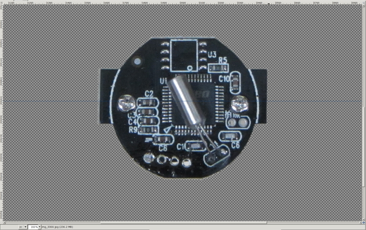
Flip back to normal view, invert the selection (to select the background, not the PCB), and delete the background to isolate the PCB:
Camera PCB – isolated – scaled
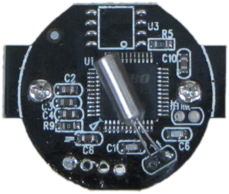
Tight-crop the PCB and flatten the image to get a white background:
Camera PCB – isolated – scaled
Fetch some digital graph paper from your favorite online source. The Multi-color (Light Blue / Light Blue / Light Grey) Multi-weight (1.0×0.6×0.3 pt) grid (1 / 2 / 10) works best for me, but do what you like. Get a full Letter / A4 size sheet, because it’ll come in handy for other projects.
Open it up (converting at 300 dpi), turn it into a layer atop the PCB image, use the color-select tool to select the white background between the grid lines, then delete the selection to leave just the grid with transparency:
Camera PCB with grid overlay – unscaled
We want one minor grid square to be 1×1 mm on the PCB image, sooo…
Accurately measure a large feature on the real physical object: 27.2 mm across the tabs
Drag the grid to align a major line with one edge of the PCB
Count the number of minor square across to the other side of the image: 29.5
Scale the grid overlay layer by image/physical size: 1.085 = 29.5/27.2
Drag the grid so it’s neatly centered on the object (or has a major grid intersection somewhere useful)
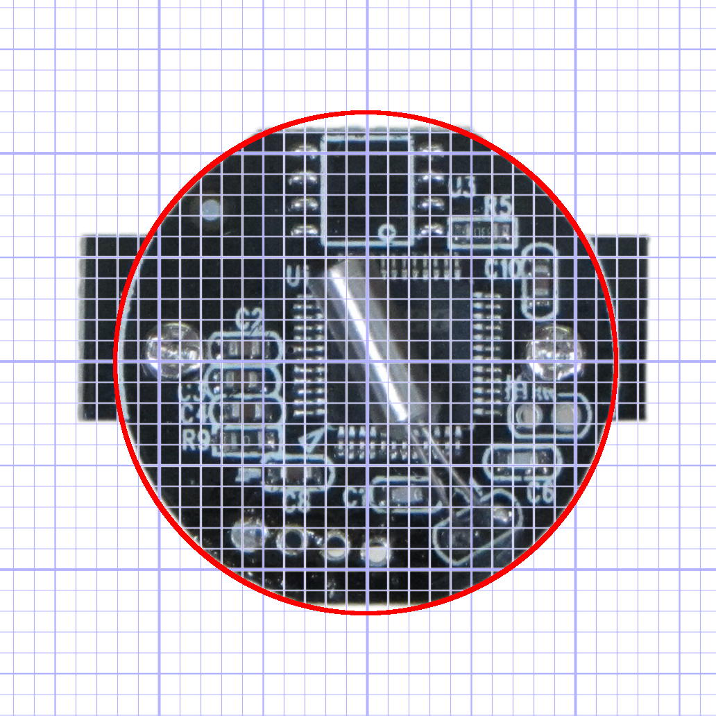
That produces a calibrated overlay:
Camera PCB with grid overlay
Then it’s just a matter of reading off the coordinates, with each minor grid square representing 1.0 mm in the real world, and writing some OpenSCAD code…
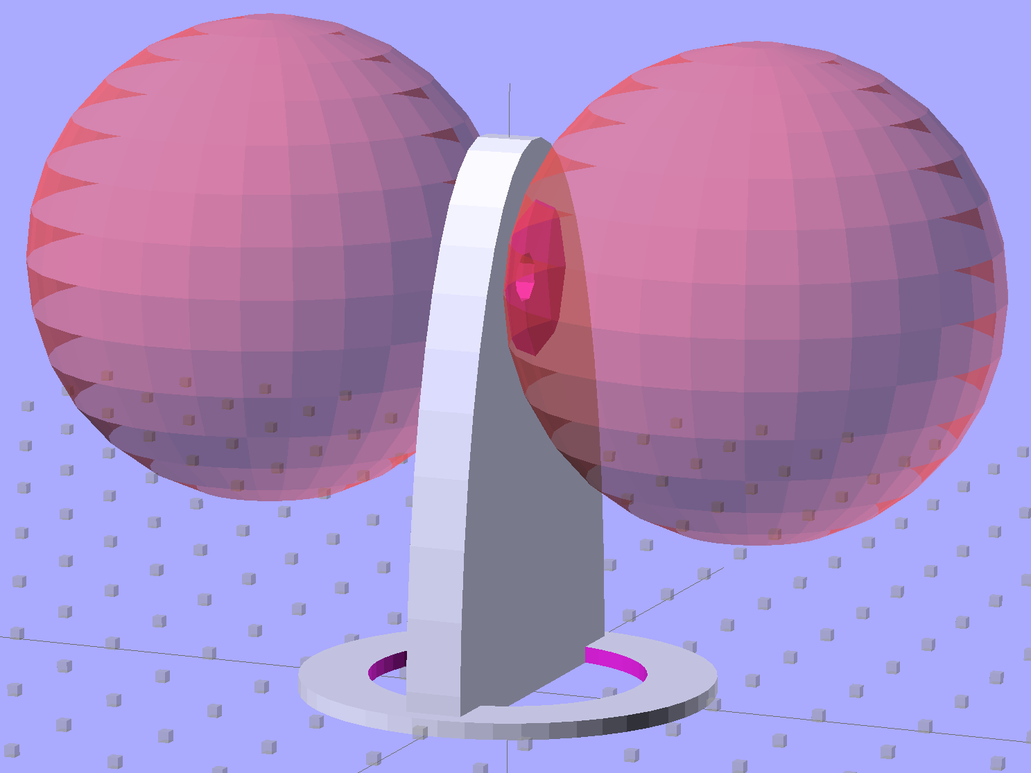
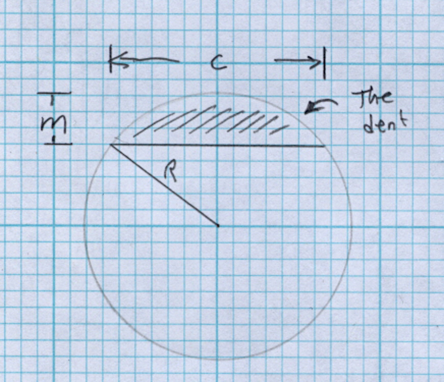
Then generate the sphere (well, two spheres, one for each dent) and offset it to scoop out the dent:
for (i=[-1,1]) {
	translate([i*(DentSphereRadius + HandleThick/2 - DentDepth),0,StringHeight])
		sphere(r=DentSphereRadius);
HandleThick controls exactly what you’d expect. StringHeight sets the location of the hole punched through the handle for a string, which is also the center of the dents.
The spheres have many facets, but only a few show up in the dent. I like the way the model looks, even if the facets don’t come through clearly in the plastic:
Quilting circle template – handle dent closeup – solid model
It Just Works and the exact math produces a better result than by-guess-and-by-gosh positioning.
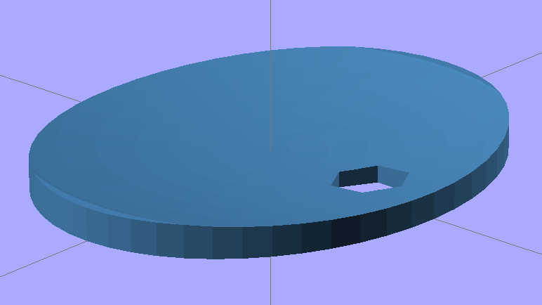
The sphere radius will come out crazy large for very shallow dents. Here’s the helmet plate for my Bicycle Helmet Mirror Mount, which has an indentation (roughly) matching the curve on the side of my bike helmet:
Helmet mirror mount – plate
Here’s the sphere that makes the dent, at a somewhat different zoom scale:
Helmet mirror mount – plate with sphere
Don’t worry: trust the math, because It Just Works.
You find equations like that in Thomas Glover’s invaluable Pocket Ref. If you don’t have a copy, fix that problem right now; I don’t get a cut from the purchase, but you’ll decide you owe me anyway. Small, unmarked bills. Lots and lots of small unmarked bills…
I put the XY coordinate origin in the middle of the platform, so that laying objects out for printing doesn’t require knowing how large the platform will be: as long as the printer is Big Enough, you (well, I) can print without further attention.
The RepRap world puts the XY coordinate origin in the front left corner of the platform, so that the platform size sets the maximum printable coordinates and all printing happens in Quadrant I. This has the (major, to some folks) advantage of using only positive coordinates, while requiring an offset for each different platform.
Yes, depending on which printer software you use, you can (automagically) center objects on your platform; this is often the only way to find objects created with Trimble (formerly Google) Sketchup. I am a huge fan of knowing exactly what’s going to happen before the printing starts, so I position my solid models exactly where I want them, right from the start. For example, this OpenSCAD model of the bike helmet mirror parts laid out for printing:
Helmet mirror mount – 3D model – Show layout
… exactly matches the plastic on the Thing-O-Matic’s platform, with the XY origin right down the middle of the platform:
Helmet mirror mount on build platform – smaller mirror shaft
It’d print exactly the same, albeit with more space around the edges, on the M2’s platform.
Similarly, the Z axis origin sits exactly on the surface of the platform. That way, the Z axis coordinate equals the actual height of the current thread extrusion in a measurable way: when you set the Z axis to, say, 2.0 mm, you can measure that exact distance between the extruder nozzle and the platform:
Taper gauge below nozzle
Now, admittedly, I fine-tune that distance by measuring the height of the skirt thread around the printed object, but the principle remains: a thread printed on the platform with Z=0.25 should be exactly 0.25 mm thick.
The start.gcode file handles all that:
;-- Slic3r Start G-Code for M2 starts --
;  Ed Nisley KE4NZU - 15 April 2013
M140 S[first_layer_bed_temperature]	; start bed heating
G90				; absolute coordinates
G21				; millimeters
M83				; relative extrusion distance
M84				; disable stepper current
G4 S3			; allow Z stage to freefall to the floor
G28 X0			; home X
G92 X-95			; set origin to 0 = center of plate
G1 X0 F30000		; origin = clear clamps on Y
G28 Y0			; home Y
G92 Y-127 		; set origin to 0 = center of plate
G1 Y-125 F30000	; set up for prime at front edge
G28 Z0			; home Z
G92 Z1.0			; set origin to measured z offset
M190 S[first_layer_bed_temperature]	; wait for bed to finish heating
M109 S[first_layer_temperature]	; set extruder temperature and wait
G1 Z0.0 F2000		; plug extruder on plate
G1 E10 F300		; prime to get pressure
G1 Z5 F2000		; rise above blob
G1 X5 Y-122 F30000	; move away from blob
G1 Z0.0 F2000		; dab nozzle to remove outer snot
G4 P1			; pause to clear
G1 Z0.5 F2000		; clear bed for travel
;-- Slic3r Start G-Code ends --
The wipe sequence, down near the bottom, positions the extruder at the front center edge of the glass plate, waits for it to reach the extrusion temperature, then extrudes 10 mm of filament to build up pressure behind the nozzle. The blob generally hangs over the edge of the platform and usually doesn’t follow the nozzle during the next short move and dab to clear the mess:
M2 – Wipe blobs on glass platform
I’ve also configured Slic3r to extrude at least 25 mm of filament in at least three passes around the object. After that, the extruder pressure has stabilized and the first layer of the object begins properly.
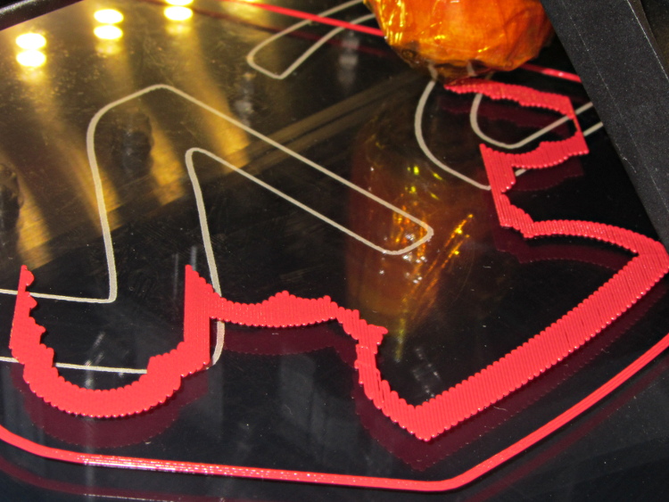
Which brings up another difference: the first layer printed on the platform is exactly like all the others. It’s not smooshed to get better adhesion or overfilled to make the threads stick together:
Robot cookie cutter – printing first layer
I print the first layer at 25 mm/s to give the plastic time to bond to the platform and use hairspray to make PLA stick to glass like it’s glued down.
I think the exported config.ini file corresponds to the currently selected set of sub-configurations; I find it difficult to keep a myriad of selections up-to-date while tweaking things, so mostly I don’t bother with named configurations.
The start.gcode and end.gcode lines go on forever, with embedded newlines.
# generated by Slic3r 0.9.11-dev on Mon Jul 22 09:28:22 2013
avoid_crossing_perimeters =
bed_size = 190,250
bed_temperature = 70
bottom_solid_layers = 3
bridge_acceleration = 0
bridge_fan_speed = 100
bridge_flow_ratio = 1
bridge_speed = 150
brim_width = 0
complete_objects = 0
cooling = 1
default_acceleration = 0
disable_fan_first_layers = 0
duplicate = 1
duplicate_distance = 6
duplicate_grid = 1,1
end_gcode = ;-- Slic3r End G-Code for M2 starts --\n;  Ed Nisley KE4NZU - March 2013\nM104 S0		; drop extruder temperature\nM140 S0		; drop bed temperature\nM106 S0		; bed fan off\nG1 Z180 F2000	; lower bed\nG1 X0 Y0 F30000	; center nozzle\nM84     	; disable motors\n;-- Slic3r End G-Code ends --
external_perimeter_speed = 50
external_perimeters_first = 0
extra_perimeters = 1
extruder_clearance_height = 20
extruder_clearance_radius = 20
extruder_offset = 0x0
extrusion_axis = E
extrusion_multiplier = .99
extrusion_width = 0.40
fan_always_on = 0
fan_below_layer_time = 45
filament_diameter = 1.72
fill_angle = 45
fill_density = 0.15
fill_pattern = honeycomb
first_layer_bed_temperature = 70
first_layer_extrusion_width = 0
first_layer_height = 100%
first_layer_speed = 25
first_layer_temperature = 175
g0 = 0
gap_fill_speed = 50
gcode_arcs = 0
gcode_comments = 0
gcode_flavor = reprap
infill_acceleration = 0
infill_every_layers = 1
infill_extruder = 1
infill_extrusion_width = 0
infill_first = 1
infill_only_where_needed = 1
infill_speed = 125
layer_gcode =
layer_height = 0.25
max_fan_speed = 100
min_fan_speed = 45
min_print_speed = 15
min_skirt_length = 25
notes =
nozzle_diameter = 0.35
only_retract_when_crossing_perimeters = 1
output_filename_format = [input_filename_base].gcode
overhangs = 1
perimeter_acceleration = 0
perimeter_extruder = 1
perimeter_extrusion_width = 0
perimeter_speed = 100
perimeters = 1
post_process =
print_center = 0,0
raft_layers = 0
randomize_start = 1
resolution = 0
retract_before_travel = 0.5
retract_layer_change = 0
retract_length = 1
retract_length_toolchange = 5
retract_lift = 0
retract_restart_extra = 0
retract_restart_extra_toolchange = 0
retract_speed = 80
rotate = 0
scale = 1
skirt_distance = 5
skirt_height = 1
skirts = 3
slowdown_below_layer_time = 20
small_perimeter_speed = 25
solid_fill_pattern = rectilinear
solid_infill_below_area = 15
solid_infill_every_layers = 0
solid_infill_extrusion_width = 0
solid_infill_speed = 100
spiral_vase = 0
start_gcode = ;-- Slic3r Start G-Code for M2 starts --\n;  Ed Nisley KE4NZU - 15 April 2013\nM140 S[first_layer_bed_temperature]	; start bed heating\nG90				; absolute coordinates\nG21				; millimeters\nM83				; relative extrusion distance\nM84				; disable stepper current\nG4 S3			; allow Z stage to freefall to the floor\nG28 X0			; home X\nG92 X-95			; set origin to 0 = center of plate\nG1 X0 F30000		; origin = clear clamps on Y\nG28 Y0			; home Y\nG92 Y-127 		; set origin to 0 = center of plate\nG1 Y-125 F30000	; set up for prime at front edge\nG28 Z0			; home Z\nG92 Z1.0			; set origin to measured z offset\nM190 S[first_layer_bed_temperature]	; wait for bed to finish heating\nM109 S[first_layer_temperature]	; set extruder temperature and wait\nG1 Z0.0 F2000		; plug extruder on plate\nG1 E10 F300		; prime to get pressure\nG1 Z5 F2000		; rise above blob\nG1 X5 Y-122 F30000	; move away from blob\nG1 Z0.0 F2000		; dab nozzle to remove outer snot\nG4 P1			; pause to clear\nG1 Z0.5 F2000		; clear bed for travel\n;-- Slic3r Start G-Code ends --
start_perimeters_at_concave_points = 1
start_perimeters_at_non_overhang = 1
support_material = 0
support_material_angle = 0
support_material_enforce_layers = 0
support_material_extruder = 1
support_material_extrusion_width = 0
support_material_interface_layers = 0
support_material_interface_spacing = 0
support_material_pattern = rectilinear
support_material_spacing = 2.5
support_material_speed = 125
support_material_threshold = 0
temperature = 175
thin_walls = 1
threads = 2
toolchange_gcode =
top_infill_extrusion_width = 0
top_solid_infill_speed = 50
top_solid_layers = 3
travel_speed = 250
use_relative_e_distances = 0
vibration_limit = 0
wipe = 0
z_offset = 0
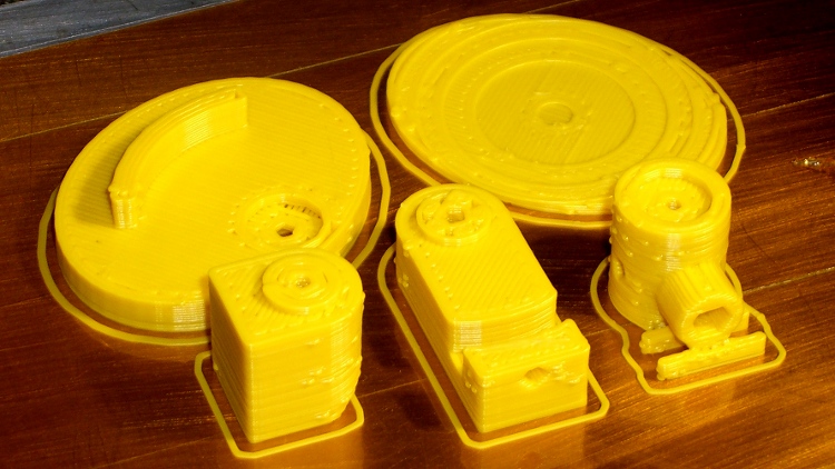
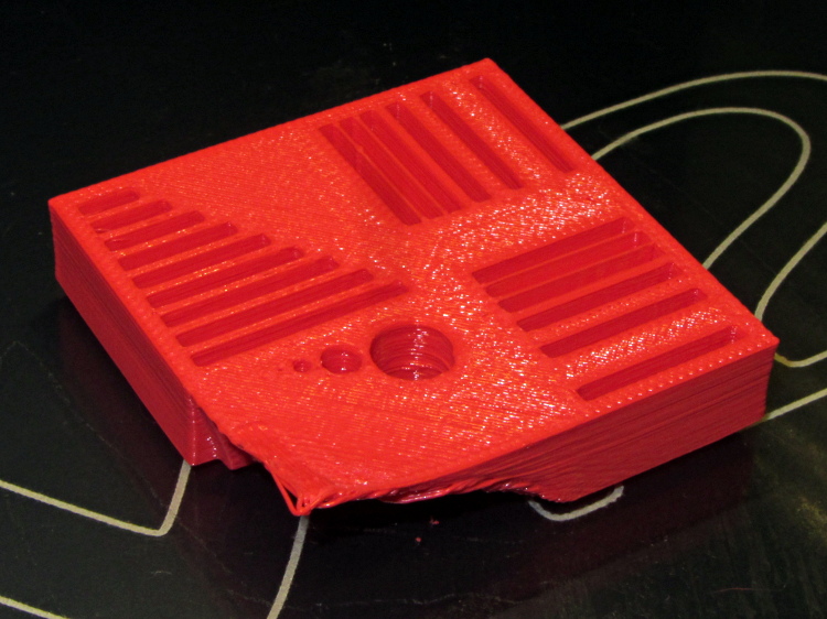
While pulling together a talk on OpenSCAD modeling (more on this later), I ran off a batch of calibration and “torture test” objects, with the intent of seeing how my somewhat modified M2 performs. The short answer is that you (well, I) can’t ask for anything better…
That level of as-printed cleanliness is typical: no stringing, no hair, no misplaced globs, no retraction problems. Basically, the plastic shape on the platform matches the mathematical shape on screen.
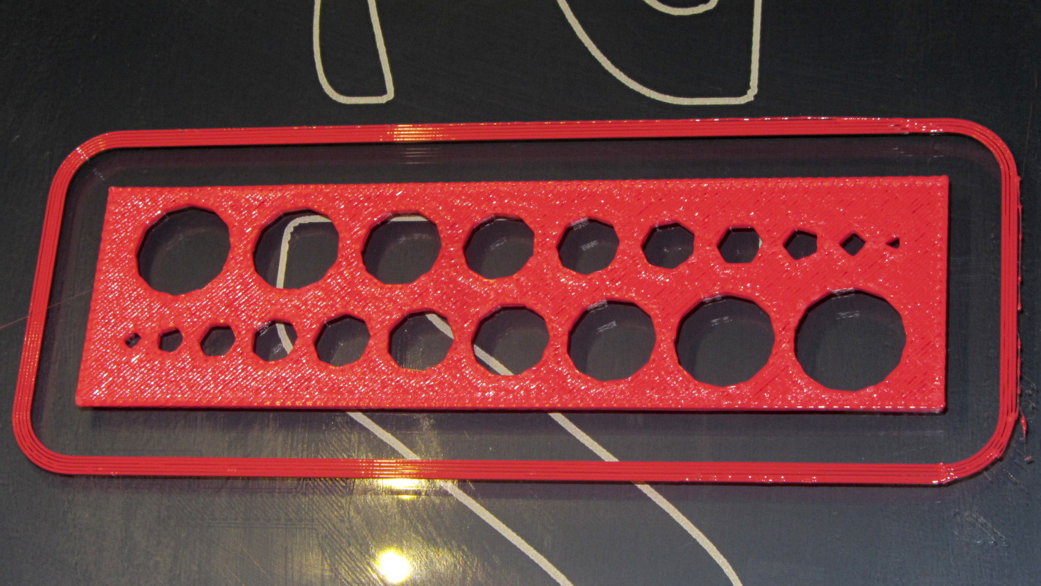
All of the linear features are with ±0.1 mm of nominal; both the 0.5 and 0.25 mm walls came out at 0.40 mm, because that’s the thread width. Slic3r doggedly puts a thread down the middle of hair-fine walls, which I think is a Good Thing.
The holes came out less than 0.3 mm undersize, which is about what you’d expect because they’re not pre-distorted and have far too many sides. The 1.0 and 0.5 mm diameter holes are present, but just barely visible; those simply aren’t reasonable sizes for this technology.
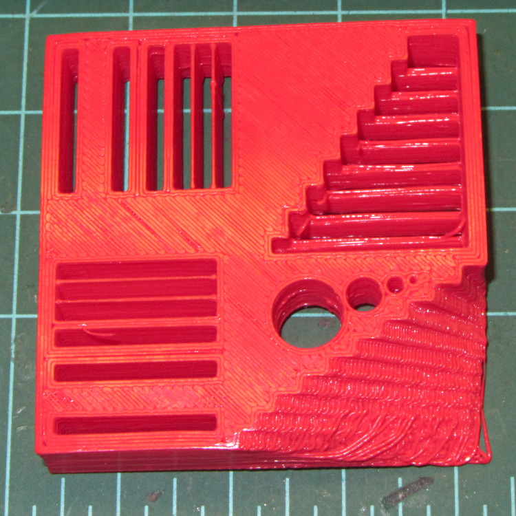
The bottom view shows a few strings in the bridge test area and more detail of the overhang:
M2 – Calibration Block – bottom
Grouping the overhangs like that produced a flat surface that tended to curl upward, so the final slopes don’t match the design. In round numbers, the M2 can handle something like a 60° overhang reasonably well.
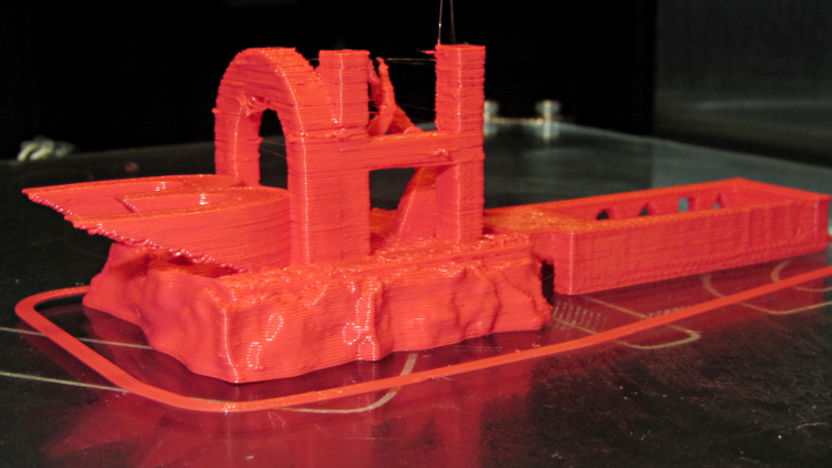
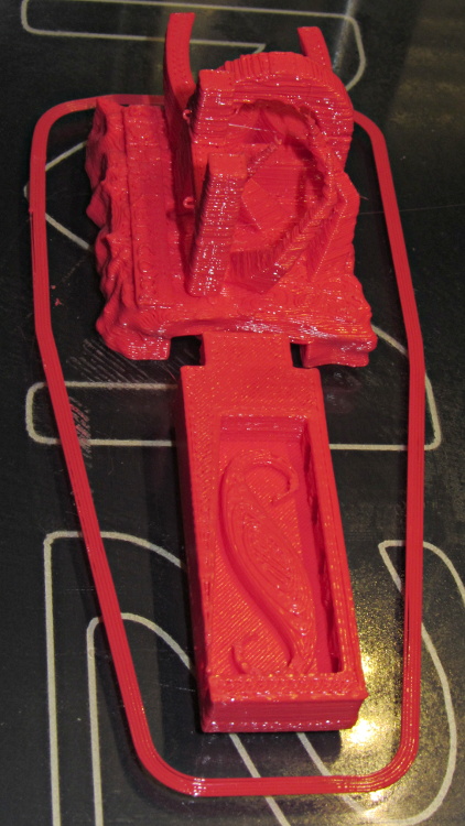
The top view shows the shape in the box looks fine, but with some curls in the main structure. The arch closed over a few random strands, so it’s rougher than I’d like:
M2 – 3DHacker object – top
The spires are lumpy and there’s more striation than I’d like, but this lies well outside the realm of stuff that I build. If I were doing it for real, I’d add some support structures here & there.
A box of surplus Vexta NEMA 23 stepper motors arrived:
Vexta C6925-9212K stepper motors
The data plate sayeth:
Model C6925-9212K
2 phase
1.8°/step
2.3 V
3 A
According to Dan, who happened into the deal, that Vexta model number applies to their custom motors, which accounts for the fact that there’s no further data available anywhere.
Dividing 2.3 V by 3 A = 0.77 Ω windings. Multiplying 2.3 V by 2 A suggests a 7 W maximum dissipation.
Poking around with a meter identifies the windings:
Blue – White – Red
Green – Yellow – Black
Given those colors, the Y G B W R K color sequence on the connector doesn’t make any sense to me. Most likely, there’s a standard I’m unaware of.
The resistance from the center taps outward measures 1.0 Ω, which is close enough to 0.8 Ω for me. Measuring across the whole winding gives 1.8 Ω.
The inductance is 1.0 mH from the center tap and 4.0 mH across the whole winding. Remember that inductance varies as the square of the number of turns.
The time constant for a complete winding = 2.5 ms = 4 mH / 1.6 Ω.