The Smell of Molten Projects in the Morning

Ed Nisley's Blog: Shop notes, electronics, firmware, machinery, 3D printing, laser cuttery, and curiosities. Contents: 100% human thinking, 0% AI slop.

Category: Software

General-purpose computers doing something specific

  • Kenmore 158: Foot Pedal Foot Bushings

    As you’d expect, the soft feet on the bottom of the Kenmore Model 158 sewing machine’s foot pedal control turn into hard buttons after a few decades. The OEM feet have mushroom tops that push through holes in the case and latch in place; of course, none of the rubber feet in my collection match the hole diameter or case thickness.

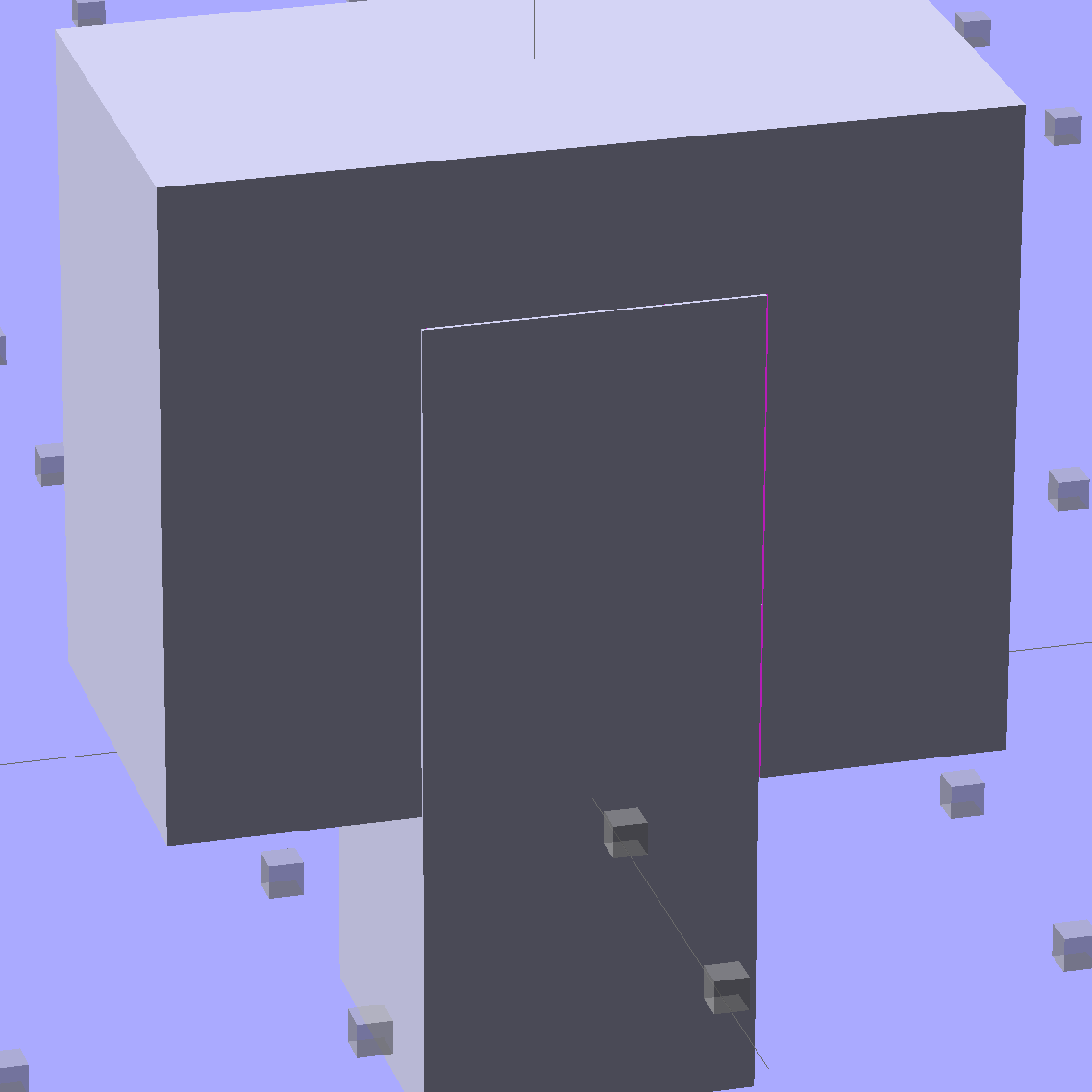
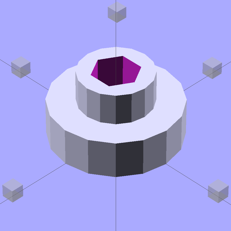
    No problem! Design a bushing that fits the case hole and passes a 4-40 screw:

    Speed Control Foot Bushing
    Speed Control Foot Bushing

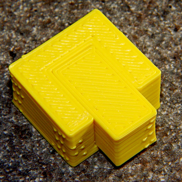
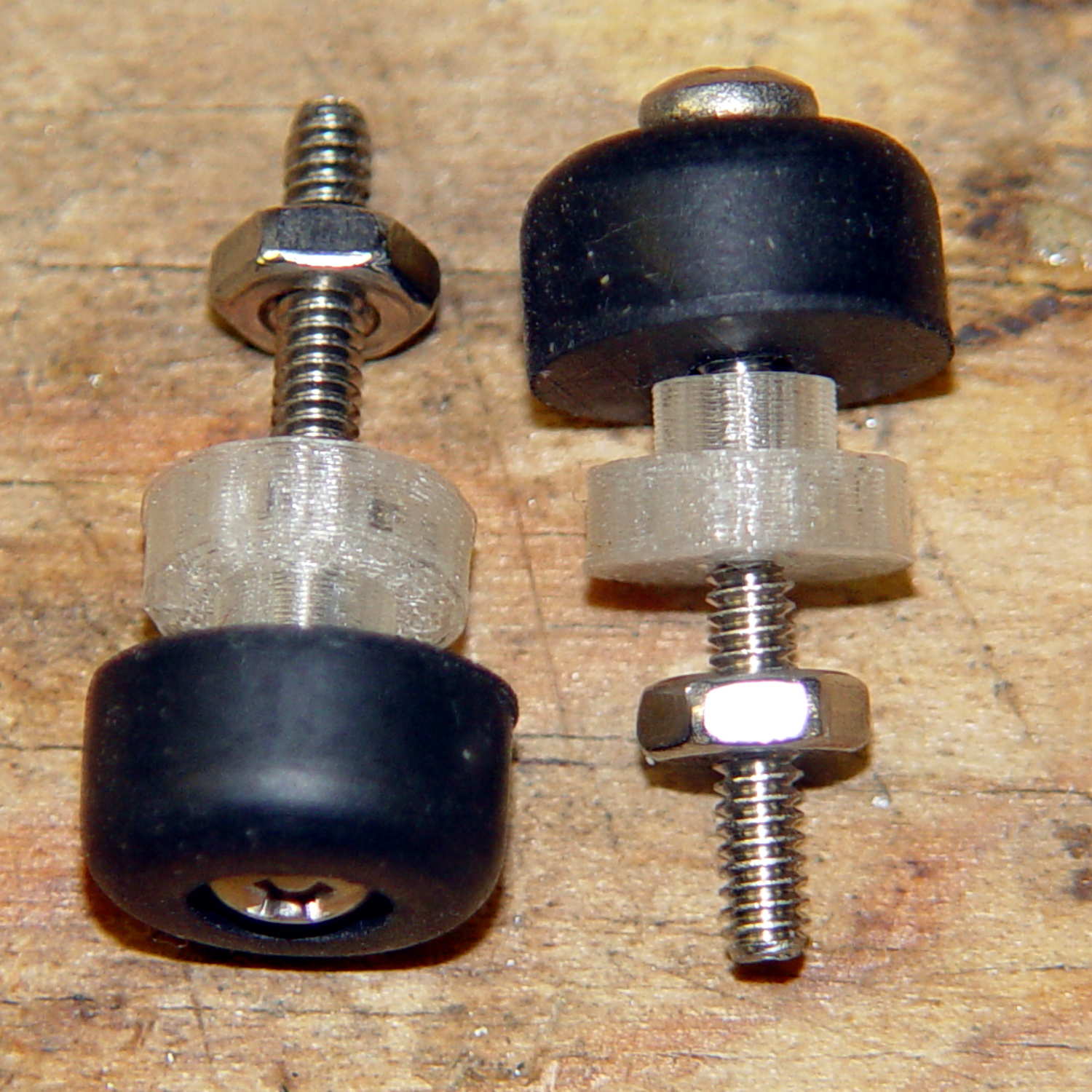
    Then print up a handful, add screws to fit the rubber feet, and top off with nuts:

    Kenmore 158 - pedal foot bushing - detail
    Kenmore 158 – pedal foot bushing – detail

    Installed, with the screws cropped to a suitable length, they look about like you’d expect:

    Kenmore 158 - pedal foot bushing - interior
    Kenmore 158 – pedal foot bushing – interior

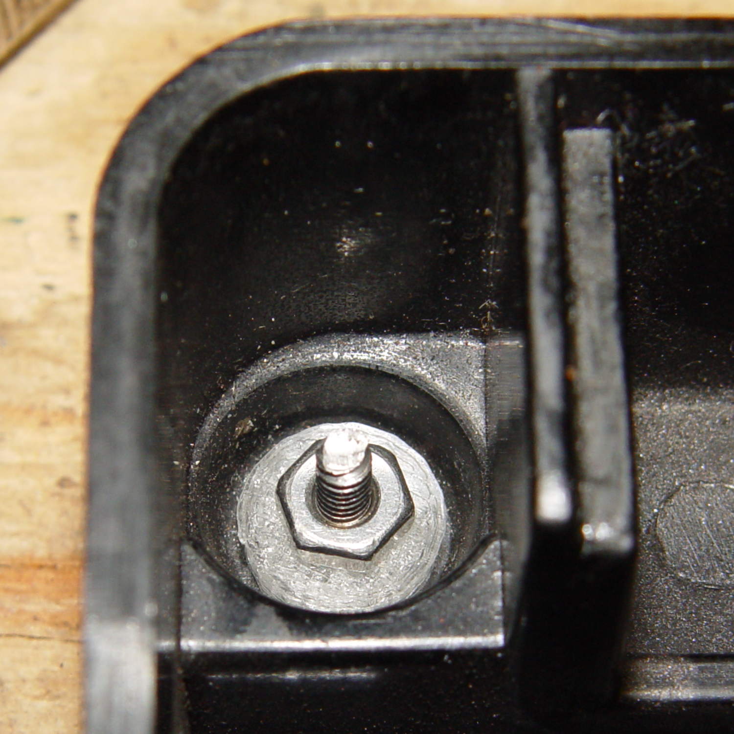
    Turns out that the springs supporting the foot pedal rest in those pockets, so the bushing reduces the spring travel by a few millimeters. The springs aren’t completely compressed with the pedal fully depressed, so it’s all good.

    The OpenSCAD source code:

    // Kenmore Model 158 Sewing Machine Foot Control Bushings
    // Ed Nisley - KE4ZNU - June 2014
    
    //- Extrusion parameters must match reality!
    //  Print with 2 shells and 3 solid layers
    
    ThreadThick = 0.20;
    ThreadWidth = 0.40;
    
    HoleWindage = 0.2;			// extra clearance
    
    Protrusion = 0.1;			// make holes end cleanly
    
    function IntegerMultiple(Size,Unit) = Unit * ceil(Size / Unit);
    
    //----------------------
    // Dimensions
    
    Stem = [2.5,5.7];			// through the case hole
    Cap = [3.0,10.0];			// inside the case
    
    LEN = 0;
    DIA = 1;
    
    OAL = Stem[LEN] + Cap[LEN];
    
    ScrewDia = 2.8;				// 4-40 generous clearance
    
    //----------------------
    // Useful routines
    
    module PolyCyl(Dia,Height,ForceSides=0) {			// based on nophead's polyholes
    
      Sides = (ForceSides != 0) ? ForceSides : (ceil(Dia) + 2);
    
      FixDia = Dia / cos(180/Sides);
    
      cylinder(r=(FixDia + HoleWindage)/2,
               h=Height,
               $fn=Sides);
    }
    
    module ShowPegGrid(Space = 10.0,Size = 1.0) {
    
      RangeX = floor(100 / Space);
      RangeY = floor(125 / Space);
    
    	for (x=[-RangeX:RangeX])
    	  for (y=[-RangeY:RangeY])
    		translate([x*Space,y*Space,Size/2])
    		  %cube(Size,center=true);
    
    }
    
    //----------------------
    // Build it!
    
    ShowPegGrid();
    
    difference() {
    	union() {
    		cylinder(d=Stem[DIA],h=OAL,$fn=16);
    		cylinder(d=Cap[DIA],h=Cap[LEN],$fm=16);
    	}
    	translate([0,0,-Protrusion])
    		PolyCyl(ScrewDia,OAL + 2*Protrusion,6);
    }
    
  • Subaru Forester: Speed Demon!

    I finally figured out why the Forester feels so slow:

    Subaru Forester - speedometer
    Subaru Forester – speedometer

    Here in the Northeast US, the maximum legal speed anywhere is 65 mph, less than half-scale, and typical around-town speeds hit 40 mph, barely 1/4 of full scale.

    For all practical purposes, that needle barely moves during our usual trips.

    I like analog gauges to represent smoothly varying quantities that you must read at a glance, but a big digital display would actually be more useful than that thing.

    A 150 mph speedometer scale makes no sense in what’s basically a shrunken all-wheel-drive SUV, even with minimal off-road capabilities. Yes, perhaps the Forester could hit 150 mph, but why not have the scale top out around, say, 100 mph? Above that, you shouldn’t be paying much attention to the speedo, anyway.

    The Sienna’s speedo went to 110 and, to the best of my knowledge, that needle never passed 85 mph, tops. However, ordinary (and legal) driving speeds filled the lower half of the scale, with the highest useful speeds in the next quadrant beyond vertical.

    Yes, I know why the speedos sport such absurd numbers. I don’t have to like it.

    There’s a servo motor (or some such) driving the needle; calibration has been a simple matter of software for a long, long time.

    For whatever it’s worth, the Forester and the Sienna have both tachometers and automatic transmissions, a combination that converts shifting into a spectator sport. The Forester’s continuously variable transmission moves the tach needle in smooth glides, rather than abrupt jumps.

  • Fit Test Blocks for 3D Printers: OpenSCAD Version

    During one of my recent presentations, somebody asked about the accuracy of 3D printed parts, which reminded me of another member of Coasterman’s Essential Calibration Set: the perimeter width/thickness test block. Back in the day, calibrating the extruder meant getting the actual ratio of the thread width to its thickness to match the ideal value you told Skeinforge to use; being a bit off meant that the final dimensions weren’t quite right.

    But when I got it right, the Thing-O-Matic printed a test block with considerable success, despite the horrible retraction zittage:

    Perimeter Calibration Block - yellow 1.10 rpm 0.33 0.66 mm
    Perimeter Calibration Block – yellow 1.10 rpm 0.33 0.66 mm

    Alas, feeding the STL to Slic3r showed that it was grossly non-manifold, and none of the automated repair programs produced good results. Turns out it’s an STL created from a Sketchup model, no surprise there, and the newer slicers seem less tolerant of crappy models.

    Sooo, here’s a new version built with OpenSCAD:

    Fit Test Blocks - build view
    Fit Test Blocks – build view

    You get three blocks-and-plugs at once, arranged in all the useful orientations, so you can test all the fits at the same time. They come off the platform about like you’d expect:

    Fit test blocks
    Fit test blocks

    I tweaked the code to make the plugs longer than you see there; the short ones were mighty tough to pry out of those slots.

    I ran the plugs across a fine file to clean the sides, without removing any base material, and the plugs fit into the slots with a firm push. I’d do exactly the same thing for a CNC milled part from the Sherline, plus breaking the edges & corners.

    The plugs doesn’t fit exactly flush in the recesses for the two models on the right side of that first image, because the edges and corners aren’t beveled to match each other. It’s pretty close and, if it had to fit exactly, you could make it work with a few more licks of the file. The left one, printed with the slot on the top surface, fits exactly as flush as the one from the Thing-O-Matic.

    Of course, there’s a cheat: the model allows 0.1 mm of internal clearance on all sides of the plug:

    Fit Test Block - show view
    Fit Test Block – show view

    The outside dimensions of all the blocks and plugs are dead on, within ±0.1 mm of nominal. You’d want to knock off the slight flange at the base and bevel the corners a bit, but unless it must fit inside something else, each object comes off the platform ready to use.

    Feel free to dial that clearance up or down to suit your printer’s tolerances.

    The OpenSCAD source code:

    // Fit test block based on Coasterman's perimeter-wt.stl
    //	http://www.thingiverse.com/thing:5573
    //	http://www.thingiverse.com/download:17277
    // Ed Nisley - KE4ZNU - May 2014
    
    Layout = "Show";
    
    //- Extrusion parameters must match reality!
    //  Print with 2 shells and 3 solid layers
    
    ThreadThick = 0.20;
    ThreadWidth = 0.40;
    
    Protrusion = 0.1;			// make holes end cleanly
    
    function IntegerMultiple(Size,Unit) = Unit * ceil(Size / Unit);
    
    //----------------------
    // Dimensions
    
    Clearance = 0.1;
    
    PlugSize = [10.0,10.0,25.0];
    BlockSize = [25.0,13.0,20.0];
    
    PlugOffset = 10.0;
    
    //----------------------
    // Useful routines
    
    module ShowPegGrid(Space = 10.0,Size = 1.0) {
    
      RangeX = floor(100 / Space);
      RangeY = floor(125 / Space);
    
    	for (x=[-RangeX:RangeX])
    	  for (y=[-RangeY:RangeY])
    		translate([x*Space,y*Space,Size/2])
    		  %cube(Size,center=true);
    
    }
    
    module Block() {
    	difference() {
    		translate([0,0,BlockSize[2]/2])
    			cube(BlockSize,center=true);
    		translate([0,PlugSize[1] - PlugSize[1]/2 - BlockSize[1]/2,-PlugOffset])
    			Plug(Clearance);
    	}
    }
    
    module Plug(Clear = 0.0) {
    	minkowski() {
    		translate([0,0,PlugSize[2]/2])
    			cube(PlugSize,center=true);
    		if (Clear > 0.0)
    			cube(Clear,center=true);
    	}
    }
    
    //----------------------
    // Build it
    
    ShowPegGrid();
    
    if (Layout == "Block")
    	Block();
    
    if (Layout == "Plug")
    	Plug();
    
    if (Layout == "Show") {
    	Block();
    	translate([0,PlugSize[1] - PlugSize[1]/2 - BlockSize[1]/2,-PlugOffset])
    		Plug();
    }
    
    if (Layout == "Build") {
    	Block();
    	translate([0,-15,0])
    		Plug();
    
    	translate([-30,0,0]) {
    		translate([0,-BlockSize[1]/2,BlockSize[1]/2])
    			rotate([-90,0,0])
    				Block();
    		translate([-PlugSize[2]/2,-15,PlugSize[0]/2])
    			rotate([0,90,0])
    				Plug();
    	}
    
    	translate([30,0,0]) {
    		translate([0,0,BlockSize[2]])
    			rotate([180,0,180])
    				Block();
    		translate([-PlugSize[2]/2,-15,PlugSize[1]/2])
    			rotate([90,0,90])
    				Plug();
    	}
    
    }
    
  • Boneheads Raven Skull: Extruder Contamination, Continued

    The Boneheads Raven Skull demo came out reasonably well, albeit in a reduced size, on the Squidwrench Frank-o-Squid:

    TOM286 - Raven Skull on platform
    TOM286 – Raven Skull on platform

    So I ran off a full-size version on the M2 for comparison:

    Raven Skull - on M2 platform
    Raven Skull – on M2 platform

    The extruder apparently contained a gobbet of black PLA, left over from the Pink Panther Woman, that managed to hang on inside until the very tip of the beak:

    Raven Skull - beak contamination
    Raven Skull – beak contamination

    Close inspection found two black strands closer to the base of the printed parts:

    Raven Skull - black contamination
    Raven Skull – black contamination

    The rear of the skull joins the front just behind the eye sockets, where the solid bottom layers make a visible contrast with the air behind the perimeter threads elsewhere. Refraction darkens some of the threads, but the two black patches stand out clearly.

    If it weren’t natural PLA, those flaws wouldn’t be nearly so noticeable.

    Were I doing this stuff for a living, I might dedicate a hot end (or an entire extruder) to each color and be done with it.

    All in all, the printed quality is about as good as I could expect from a glorified glue gun.

    The extreme slowdown while printing the tip of the beak pushed Pronterface’s remaining time estimate over the edge:

    Boneheads - Raven - Pronterface time estimate
    Boneheads – Raven – Pronterface time estimate

    I’m not sure what the correct value should be …

  • Poughkeepsie to Rochester Road Trip: The Movie

    With the Sony HDR-AS30V camera Gorilla Taped to the Sienna’s dashboard, we drove it to Rochester with a bank shot off Saratoga:

    Saratoga Rt 50
    Saratoga Rt 50

    I then converted nearly 5000 images into Yet Another Crappy Youtube Movie that is, mercifully, only 00:02:43 long.

    The key steps:

    mkdir /tmp/Video
    cd /tmp/Video
    sn=1 ; for f in /mnt/backup/Video/2014-05-29/* ; do printf -v dn 'dsc%05d.jpg' "$(( sn++ ))" ; cp -a $f $dn ; done
    avconv -r 30 -i dsc%05d.jpg -q 5 Pok-Saratoga-Rochester.mp4
    

    I tossed out a few images you didn’t need to see, then renumbered the remainder:

    sn=1 ; for f in * ; do printf -v dn 'dsc%05d.jpg' "$(( sn++ ))" ; mv $f $dn ; done
    

    The point of this exercise was to find out how Youtube treats “HD” movies. The original 1920×1080 MP4 file weighed in at nearly 500 MB with very good quality (due to the -q 5), but the Youtube “HD” result exhibits terrible compression artifacts; the black cloth crawls with huge checkerboard squares. Because the relatively slow-moving sequences at traffic signals and rest stops have excellent quality, I’d say Youtube’s video bit rate just doesn’t support images that change completely from frame to frame. Makes sense; nobody could watch such a thing, so why allocate that many bits?

    Now I have another Youtube movie-making data point

  • Twiddling Linux Swap Performance

    Depending on a solid model’s complexity, OpenSCAD will sometimes chew through system memory, consume the entire swap file, and then fall over dead. In an attempt to work around that situation, I recently jammed a 32 GB USB drive into the back of the box, turned it into a swap device, and then told the kernel to back off its enthusiasm for swapping.

    Format the USB drive as a swap device:

    sudo mkswap /dev/sd??   #--- unmount it before you do this!
    Setting up swapspace version 1, size = 31265292 KiB
    no label, UUID=0f559a8c-67b7-4fa3-a709-17aeec3104c4
    

    Add it to /etc/fstab and set swap priorities:

    # swap was on /dev/sdb3 during installation
    UUID=e8532714-ad80-4aae-bee7-a9b37af63c8c none  swap sw,pri=1	0 0
    UUID=0f559a8c-67b7-4fa3-a709-17aeec3104c4 none	swap sw,pri=5	0 0
    

    Turn it on:

    sudo swapon -a
    

    Following those directions, dial back the kernel’s swappiness and limit the file cache growth:

    sudo sysctl -w vm.swappiness=1
    sudo sysctl -w vm.vfs_cache_pressure=50
    

    Those commands now live in /etc/sysctl.d/99-swappiness.conf:

    cat /etc/sysctl.d/99-swappiness.conf
    # Improve responsiveness by reducing cache swapping
    vm.swappiness=1
    vm.vfs_cache_pressure=50
    

    For whatever reason, WordPress turns underscores into blanks, so those obvious typos aren’t, really.

    And then it should Just Work.

    The box has 4 GB of RAM and, under normal circumstances, doesn’t swap at all, so I expect the USB drive should kick in only for extreme OpenSCAD models. The swappiness tuning should help during ordinary operation with large file operations.

    I have no results to report, but if something blows up, I know what changed…

  • Hall Effect LED Current Control: Crisp Gate Drive Shaping

    Because the current control loop closes through the Arduino loop(), the code’s path length limits the bandwidth. Worse, the PWM filter imposes a delay while the DC value catches up with the new duty cycle. Here’s what that looks like:

    LoopStatus ILED 50 mA div - 200 50 150 25 mA
    LoopStatus ILED 50 mA div – 200 50 150 25 mA

    The setpoint current for this pulse is 200 mA, ramping upward from 50 mA. It should have started from 25 mA, but the loop really wasn’t under control here.

    The top trace goes low during the drain current measurement, which occurs just before the code nudges the gate drive by 1 PWM count to reduce the error between the setpoint and the measurement. A delay(1) after each PWM change, plus the inherent delay due to all the program statements, produces an update every 1.7 ms, more or less.

    Even at that low rate, the current overshoots by 50 mA before the loop can tamp it down again. The current varies by 200 mA for 7 PWM counts, call it 30 mA per count at the high end, so overshooting by 50 mA comes with the territory. There’s just not a lot of resolution available.

    The program reads each pulse duration and amplitude from an array-of-structs, so it’s a simple matter of software to save the gate drive voltage at the end of each pulse and restore it when that pulse comes around on the guitar again:

    	if (millis() >= (EventStart + (unsigned long)Events[EventIndex].duration)) {
    		Events[EventIndex].drive_a = VGateDriveA;						// save drive voltages
    		Events[EventIndex].drive_b = VGateDriveB;
    
            if (++EventIndex > MAX_EVENT_INDEX)								// step to next event
    		    EventIndex = 0;
    
    		VGateDriveA = Events[EventIndex].drive_a;						// restore previous drives
    		VGateDriveB = Events[EventIndex].drive_b;
    
    		SetPWMVoltage(PIN_SET_VGATE_A,VGateDriveA);
    		SetPWMVoltage(PIN_SET_VGATE_B,VGateDriveB);
    
    		delay(PWM_Settle);
    
    		digitalWrite(PIN_ENABLE_A,Events[EventIndex].en_a);				// enable gates for new state
    		digitalWrite(PIN_ENABLE_B,Events[EventIndex].en_b);
    
            NeedHallNull = !(Events[EventIndex].en_a || Events[EventIndex].en_b);	// null sensor if all off
    
    		EventStart = millis();                                          // record start time
    	}
    

    … which produces this happy result, with a different time scale to show all four pulses in the array:

    I Sense Amp  ILED 50 mA div - 200 100 150 50 mA
    I Sense Amp ILED 50 mA div – 200 100 150 50 mA

    The top trace shows the current amp output that goes into the Arduino analog input and the bottom trace shows the MOSFET drain current. Notice those nice, crisp edges with a nearly complete lack of current adjustment.

    The small bumps in the amp output just after the LED turns off happen while the the code nulls the Hall effect sensor offset. Whenever the LEDs turn off, the code nulls the sensor, which is probably excessive; it really doesn’t have much else to do, so why not?

    This trickery doesn’t improve the loop bandwidth at all, because the code must still drag the current to meet each setpoint, but now that happens only when the pulse first appears. After a few blinks, the current stabilizes at the setpoint and the loop need handle only slight variations due to temperature or battery voltage changes.

    Speaking of voltages:

    VDS ILED 50 mA div - 200 100 150 50 mA
    VDS ILED 50 mA div – 200 100 150 50 mA

    The top trace now shows the MOSFET drain voltage and the bottom still has the LED current. There’s only 650 mV of difference at the drain for currents of 50 mA and 200 mA through the LEDs, with about 1 V of headroom remaining at 200 mA.

    The power supply delivers 7.4 V to the anode end of the LEDs, so they drop 6.3 V @ 200 mA and 5.7 V @ 50 mA. Some informal knob twiddling suggests that the MOSFET loses control authority at about 6.5 V, so, given that there’s not much energy in the battery below 7.0 V anyway, the program could limit the  maximum current to 50 mA when the battery hits 7 V, regain 650 mV of headroom, and run at reduced brightness (and perhaps a different blink pattern) until the battery drops to 6.5 V, at which point the lights go out.

    There’s more improvement to be had in the code, but those pulses look much better.

    (If you’re keeping track, as I generally don’t, this is Post Number 2048: love those round numbers!)