
An addition to my morning cocoa makes it mmmm turn out better:

Start with an ounce of milk, dump in the rest of the ingredients, spin up the stirrer, and slowly add the 8 oz of milk that just reached the end of its 70 seconds in the microwave:
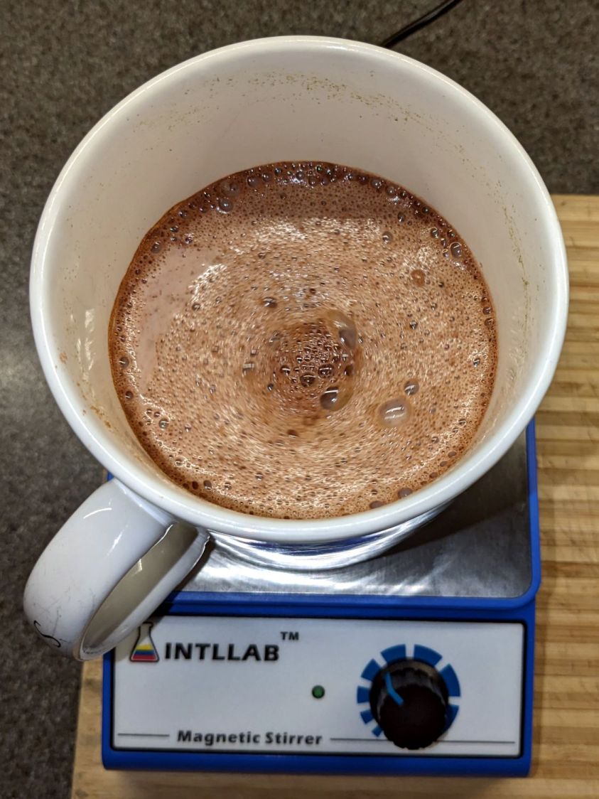
The green LED to the left of the speed knob runs from the PWM signal driving the motor, so it flickers visibly and interacts with the camera shutter.
Let it whir for a few minutes until all the cocoa bombs vanish and it’s ready for another 33 seconds in the microwave.
The most recent batch of cocoa arrived in an exceedingly vacuum-packed mylar bag, to the extent the bag resembled a brick and the solid cocoa within fractured into big chunks. Bashing the chunks with a fork got tedious enough to remind me of the stirrer I got to mix titanium dioxide for the yet-to-be-tried glass engraving.
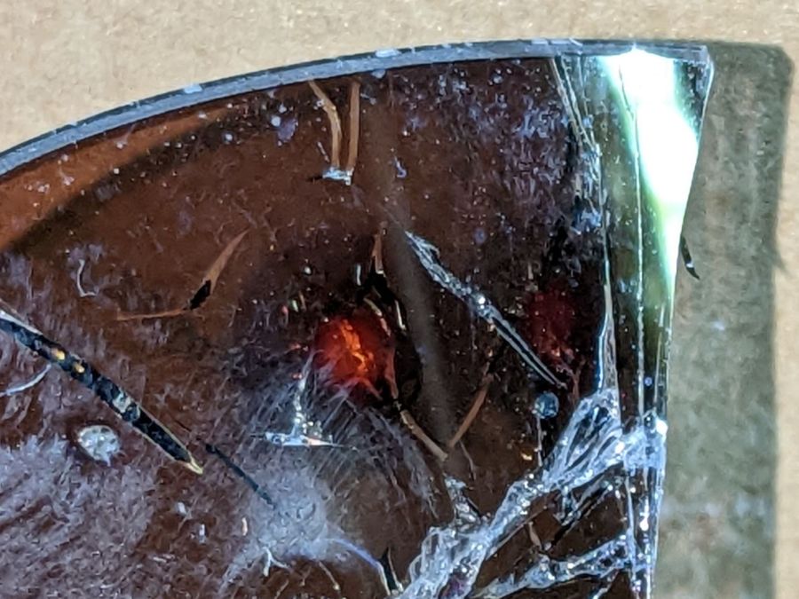
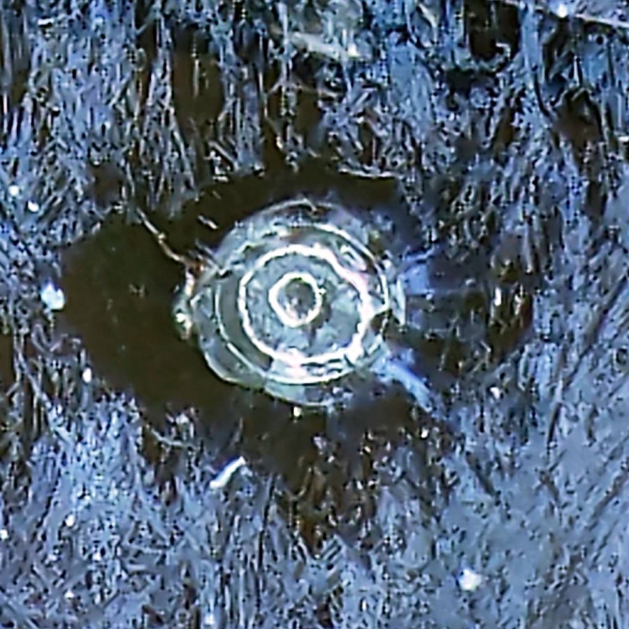
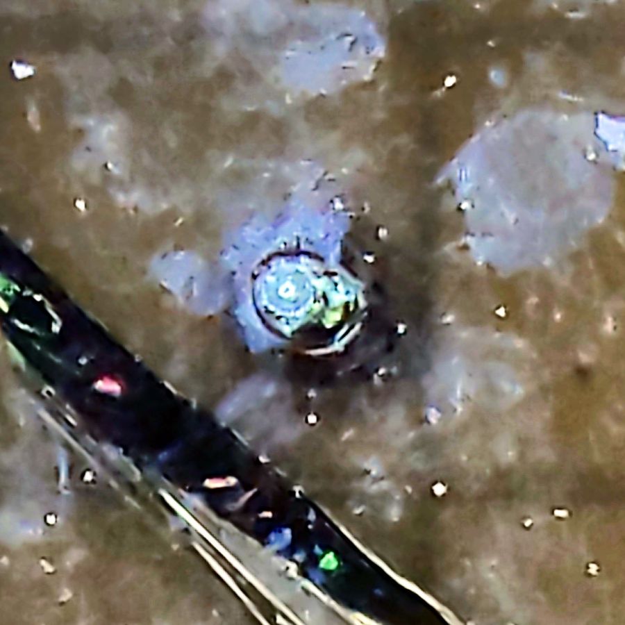
Back in the day, the teflon shell molded on the magnet had a rib around its middle to make it pivot neatly on a point contact. This one is flat and dislikes spinning on the slightly concave cup bottom.
Protip: fish the stirrer out before sipping the cocoa, lest it become a tiny cow magnet.


