Just to see what the laser tube’s output looks like, I aimed a large photodiode toward the laser tube output:
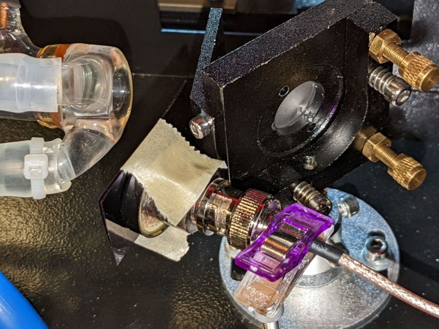
That’s a venerable PIN-10AP photodiode minus its green human-eye filter, with an IR-pass / visible-block set of gel filters taped on the front to knock out everything except IR scattered from the laser’s snout. Nothing sits in the direct beamline.
The alert reader will kvetch about a CO₂ laser running at 10.6 µm, an order of magnitude off the right end of the photodiode response curve graphs, through stage filter gels not even pretending to have optical specs. Hey, stage light filters are utterly transparent to thermal IR and there’s plenty of invisible light to go around, so maybe this will work.
The coaxial cable trails off to the scope’s 1 MΩ input, so, although the photodiode does not operate in true zero-bias mode, I can at least look at its photocurrent driving a voltage into the scope input.
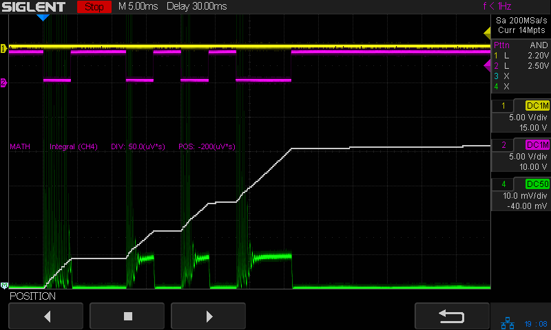
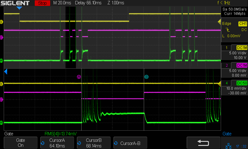
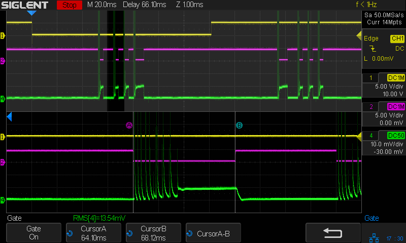
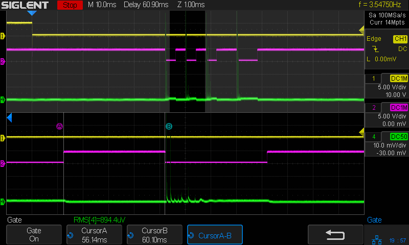
Surprisingly, the lashup kinda-sorta works well enough to show the laser’s light output tracking the tube’s current:

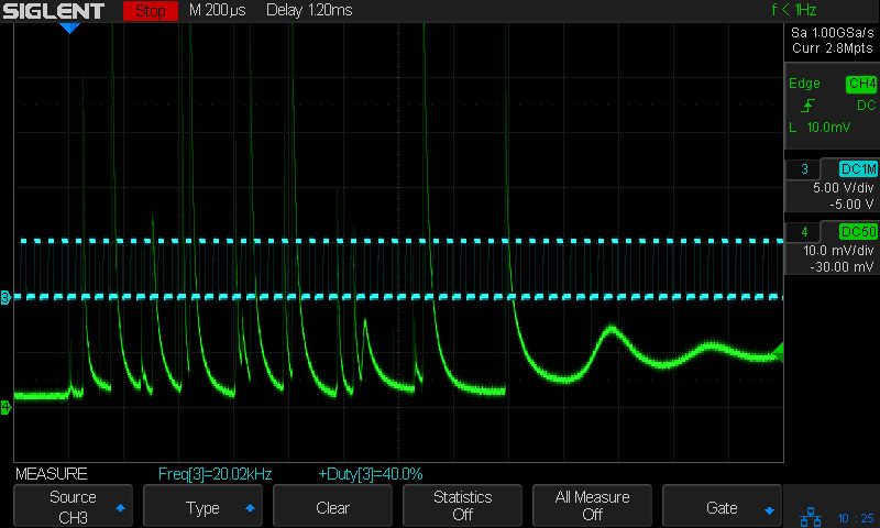
That’s a manual 20 ms pulse at 90% PWM, with the tube current at 20 mA/div. The oscillations at the start of the current pulse seem to excite the tube enough for the light output to stabilize when the real current comes along. I cannot tell if the exponential tail-off beyond the pulse is due to excited molecules cooling off in the laser tube or the poor photodiode recovering from Too. Much. Light. It. Burns.
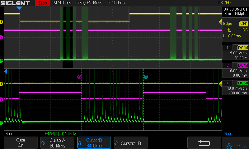
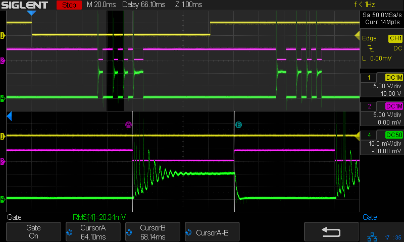
The response is a little shakier at 50% PWM:
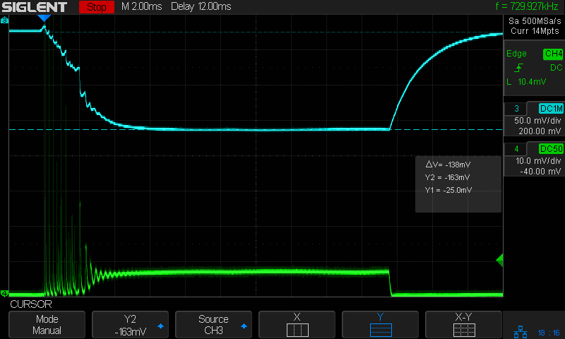
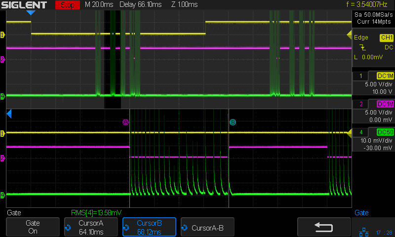
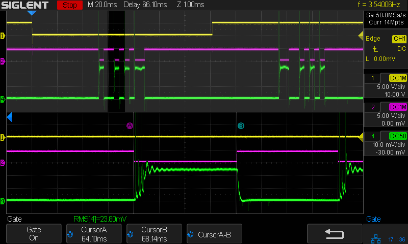
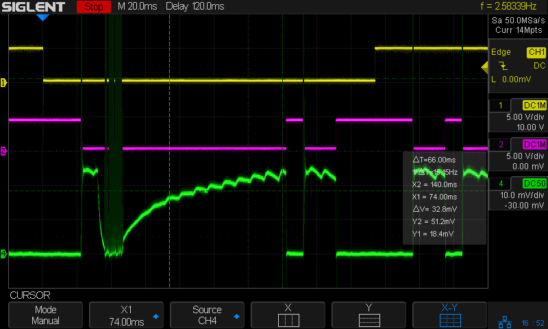
Dropping to 30% PWM requires more time to get up and running:

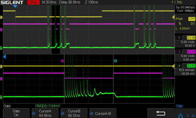
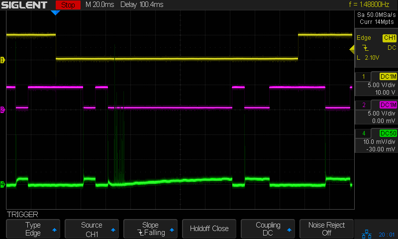
And 10% PWM looks downright awful:
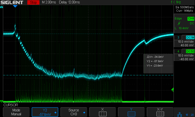
Although the vertical scale for the photodiode trace doesn’t mean much, it’s obvious that the IR output matches the current input, right down to the littlest pulses. Sliding a bit of brass shimstock between the filter gels eliminates nearly all the photodiode output, so it’s not electrical noise. I think the long tail really shows the gases cooling off.
The alert reader will have noted the wee blip over there on the right, 21 ms after the start of the 20 ms long pulse and 4 ms after all those spikes shut off. Yup, the HV power supply can deliver a stray pulse when it’s not supposed to be enabled. More on that in a while.