Category: Electronics Workbench

Electrical & Electronic gadgets

Marlin Firmware: Stepper Interrupt Timing
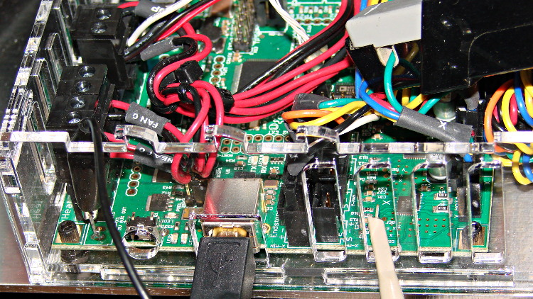
Based on the discussion attached to the post on Z axis numbers, I wanted to take a look at the points where Marlin switches from one step per interrupt to two, then to four, just to see what the timing looks like. The RAMBo board has neatly labeled test points, to which I tack-soldered a pin for the scope probe poked through one of the ventilation slots, and an unused power connector on the left edge of the PCB that provided a ground point (admittedly, much too far away for good RF grounding, but it suffices for CMOS logic signals). The Tek Hall-effect current probe leaning in from the top right captures the current in one of the X axis windings:

X axis Step and Current probes

I’ve reset the Marlin constants based on first principles, per the notes on distance, speed, and acceleration, so they’re not representative of the as-shipped M2 firmware. Recapping the XY settings:
- Distance: 88.89 step/mm
- Speed: 450 mm/s = 27000 mm/min
- Acceleration: 5000 mm/s², with the overall limit at 10 m/s²
The maximum interrupt frequency is about 10 kHz and the handler can issue zero, one, two, or four steps per axis per interrupt as required by the speed along each axis, up to a maximum of step rate of 40 kHz. There are complexities involved which I do not profess to understand.

The maximum 10 kHz step rate for one-step-per-interrupt motion corresponds to a speed of:

112.5 mm/s = (10000 step/s) / (88.89 step/mm)

The maximum 40 kHz step rate produces, naturally enough, four times that speed:

450 mm/s = (40000 step/s) / (88.89 step/mm)

Assuming constant acceleration, the distance required to reach a given speed from a standing start or to decelerate from that speed to a complete stop is:
x = v² / (2 * a)

The time required to reach that speed is:
t = v/a

Accelerating at 5000 mm/s²:
- 112.5 mm/s = 6700 mm/min → 1.27 mm, 22.5 ms
- 150 mm/s = 9000 mm/min → 2.25 mm, 30 ms
- 450 mm/s = 27000 mm/min → 20.3 mm and 90 ms
An overview of a complete 6 mm move at 150 mm/s shows the acceleration and deceleration at each end, with a constant-speed section in the middle:

X Axis 150 mm-s 6 mm – overview

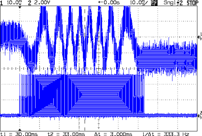
The bizarre patterns in the traces come from hp2xx‘s desperate attempts to discern the meaning of the scope’s HPGL graphic data where the trace forms a solid block of color; take it as given that there’s no information in the pattern. I described the trace conversion process there.

The upper trace shows the X axis motor winding current at a scale of 500 mA/div, with far more hash than one would expect. The RAMBo drivers evidently produce much more current noise than the brick drivers I intend to use.

The lower trace is the X axis step signal produced by the Arduino microcontroller. You can barely make out the individual step signals at each end, but there’s not enough horizontal resolution to show them when the motor moves at a reasonable pace.

In round numbers, the acceleration and deceleration should require about 30 ms each. The overall move takes 63 ms, so the constant-speed section in the middle must be about 3 ms long. That’s probably not right…

Here’s a closer look at the step pulses as the motion starts from zero on the way to 150 mm/s:

X Axis 150 mm-s 6 mm – 1 ms-div 0 ms dly

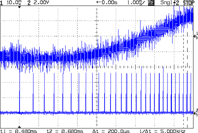
Over on the right, the 5 kHz step rate after 8.5 ms suggests a speed of 56 mm/s and counting 28 pulses says it moved 0.32 mm. Plugging those numbers into the equations:
- a = v/t = 6600 mm/s²
- a = (2 * x)/t² = 8900 mm/s²
It’s not clear (to me, anyway) whether:
- The firmware accelerates faster than the alleged 5000 mm/s² limit
- It’s accelerating near the overall limit of 10000 mm/s²
- The acceleration isn’t constant: starts high, then declines
- The measurement accuracy doesn’t support any conclusions
- I understand what’s happening
In order to see the double- and quad-step outputs, here’s a 50 mm move at 450 mm/s, with a 19 ms delay to the point where the interrupt handler transitions from single-step to double-step output:

X Axis 450 mm-s 50 mm – 200 us-div 19 ms dly

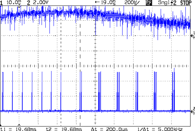
The interrupt frequency drops from just under 10 kHz to a bit under 5 kHz, with the doubled pulses about 16 μs apart. At the transition, the axis speed is 112.5 mm/s, pretty much as predicted.

If that’s the case, the overall acceleration to the transition works out to:

5800 mm/s² = (113 mm/s) / (19.5 ms)

Delaying the traces to 41.9 ms after the motion starts shows the double-to-quad step transition:

X Axis 450 mm-s 50 mm – 100 us-div 41.9 ms dly

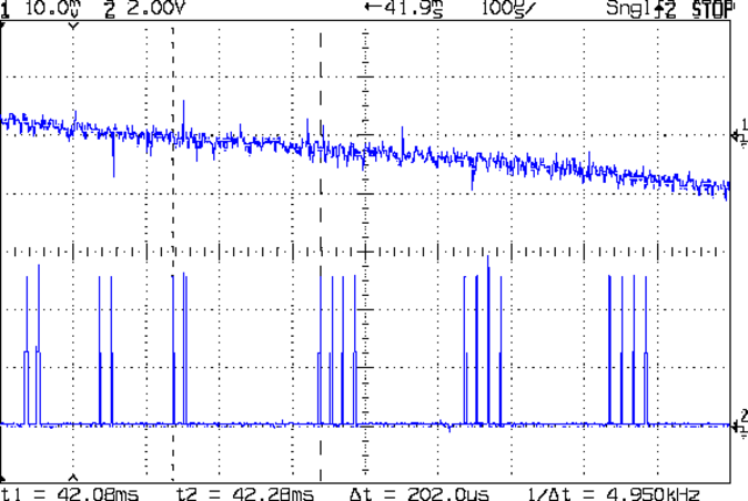
Once again, the pulse frequency drops from 10 kHz down to 5 kHz. The speed is now 225 mm/s, half the maximum possible speed, which also makes sense: at top speed, the pulses will be essentially continuous at 40 kHz.

The average acceleration from the start of the motion:

5300 mm/s² = (225 mm/s) / (42.1 ms)

That implies the initial acceleration starts higher than the limit, but it evens out on the way to the commanded speed.

Those scope shots come from moving only the X axis. Moving both the X and Y axes, with Trace 1 now showing the Y axis output, for 50 mm at 450 mm/s, produces similar results; the Y axis output lags the X axis by a few microseconds:

XY 450 mm-s 50 mm – 100 us-div 19.5 ms dly

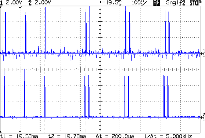
Once again, that’s at the single- to double-step transition at 19+ ms. The overall timing doesn’t depend on how many axes are moving, as long as they can accelerate at the same pace; otherwise, the firmware must adjust the accelerations to make both axes track the intended path.

None of this is too surprising.

For a motor running at a constant speed just beyond the single-to-double step transition at 112.5 mm/s or the double-to-quad transition at 225 mm/s, the rotor motion should have a 5 kHz perturbation around its nominal position: it coasts for nearly the entire period, then a pair of steps kicks it toward the proper position. At those transitions, the rotor turns at:

3.2 rev/s = (10000 step/s) / (3200 step/rev) 6.4 rev/s = (20000 step/s) / (3200 step/rev)

The perturbation should look like a 5 kHz oscillation (not exactly sinusoidal, maybe triangular?) superimposed on the nominal position, which is changing more-or-less parabolically as a function of time. I expect that the overall inertia damps it out pretty well, but I’d like to attach a rotary encoder to the motor shaft (or a linear encoder to the axis) to show the actual outcome, but I don’t have the machinery for that.

In any event, LinuxCNC’s step outputs should behave better, which is why I’m doing this whole thing in the first place…
2013-06-04
LED Output vs. Current: Efficiency Loss

Some data points from that circuit produced this graph:

LED Output vs Current

Relative to the output at 5 mA, the efficiency drops off pretty much linearly:

LED Efficiency vs Current

That’s computed as the ratio of the actual light output to the output at 5 mA scaled by the current ratio.

So putting the screws to the LEDs does produce more light, but not quite as much as you’d expect. Above maybe 40 mA, it’s not worth the effort.

Now we know…

2013-05-28
LED Driver + Zero-bias Photodiode Amplifier

This may come in handy for something, like measuring LED output:

LED Output Tester – Schematic

The LM324 converts the input voltage to an LED drive current, scaled by the sense resistor and the gain of IC2B to 25 mA/V. The feedback loop closes through the MOSFET and C6 rolls off the response, so there’s a nasty overshoot on the leading edge of input pulses where the current increases faster than the op amp can tamp it down:

Red LED – 25 mA 14 uA

The LM356 acts as a transimpedance amplifer to convert the photodiode current to voltage. The PIN-10AP specs say it should operate in photovoltaic mode with zero bias and that more than -3V of bias will kill the photodiode; the LM356 should hold its inverting input at virtual ground, but the two 1N5819 Schottky diodes enforce that limit. There being zero volts across the diodes, they don’t leak in either direction, so it’s all good.

The circuit is an embarrassing hairball on solderless breadboard, so use your imagination…

You could mash this together with the LED Curve Tracer, although you’d want better low-current resolution from the Arduino output.

2013-05-27
LED + Photodiode: Verifying Linearity

Given that test fixture, the obvious question is whether the PIN-10AP photodiode’s output current varies linearly with light intensity, just like the specs would lead you to believe. I excavated the sheet of 2-stop neutral density filter gel from the Parts Warehouse Wing and cut some 30 mm disks:

LED Photodiode test fixture – ND filter disks

A single filter layer should reduce the light intensity by 2 f/stops = a factor of 4. Each successive layer reduces the intensity by another factor of 4. They’re all at least reasonably clean and free of defects, but they’re definitely not optical lens quality.

Running the LED with a 100 mA pulse at 20% duty cycle and stacking the disks in the fixture, one by one, between the LED and photodiode, produces this data:

Layers Attenuation Scale V I – uA Ratio

0 1 1.0000 8.7 87

1 4 0.2500 1.9 19 4.58

2 16 0.0625 0.43 4.3 4.42

3 64 0.0156 0.097 0.97 4.43

4 256 0.0039 0.022 0.22 4.41

The Ratio column divides successive pairs of current values. The first step, from “no filter” to “one filter”, came out a bit larger than the rest, probably because the gel sheet isn’t anti-reflective and some light bounces off the top.

After that, though, it looks just like I’m cheating, doesn’t it?

The ratios should be 4.0, but the actual 4.4 means it’s a 2.1 stop filter. Close enough, methinks.

2013-05-24

LED + Photodiode Test Fixture

An upcoming Circuit Cellar column calls for a way to measure LED light output vs. current input, which means I need some way to hold LEDs directly over a photodiode while excluding ambient light. Fortunately, the M2 had black PLA filament already loaded:

LED Photocell Fixture - parts — LED Photocell Fixture – parts

That honkin’ big photodiode is a surplus PIN-10AP that’s been lying in wait for an opportunity just like this. The green filter matches the silicon response to CIE-standard human eye sensitivity, so the output tracks what you’d actually see. That’s irrelevant for testing red LEDs that all have pretty much the same wavelength, but it might come in handy for something.

The main body of the fixture holds the LED about 1 mm from the front of the photodiode, indexed against the LED flange so they’re all at a consistent location. The cap has three locating pins made of 3 mm orange filament, with black foam rubber to push the LED into position and block ambient light.

The business end looks like this:

LED Photocell Fixture - LED view — LED Photocell Fixture – LED view

The most convenient way to mount the thing involves a right-angle BNC adapter in my trusty bench vise:

LED Photocell Fixture - with breadboard — LED Photocell Fixture – with breadboard

The circuitry has a voltage-to-current driver for the LED and a zero-bias current-to-voltage converter for the photocell. The zero-bias trick keeps the voltage across the photodiode at zero, so the current varies linearly with illumination.

The solid model laid out for printing along the X axis:

LED Fixture for PIN-10AP Photodiode - solid model overview — LED Fixture for PIN-10AP Photodiode – solid model overview

It obviously has some improvements over the as-printed one in the pictures, in the unlikely event I need another fixture. The most important: a rear ring covering the back of the photodiode. Turns out that the PIN-10AP filter cap leaks a surprising amount of light around the body; I covered the gap with black tape to make the measurements, but that’s crude.

I added a few screw holes to hold the parts together, but the cap (with the foam and pegs) must come off easily while swapping LEDs. I’d be tempted to sink studs into the body and use wing nuts to hold the lid in place, but I don’t have any 4-40 wing nuts…

There’s a tiny bit of support under the central hole to support the LED flange recess and the trench for some foam under the leads:

LED Fixture for PIN-10AP Photodiode - support — LED Fixture for PIN-10AP Photodiode – support

That’s another improvement; the as-printed one has foam on only one side of the leads.

The OpenSCAD source code:

// LED test fixture for PIN-10AP photodiode
// Ed Nisley KE4ZNU May 2013

// Layouts: Adapter AdapterSupport Cap Shield Build Show

Layout = "Build";

Gap = 8;		// between parts in Show

//- Extrusion parameters must match reality!
//  Print with +1 shells and 3 solid layers

ThreadThick = 0.25;
ThreadWidth = 0.40;

HoleWindage = 0.2;

function IntegerMultiple(Size,Unit) = Unit * ceil(Size / Unit);

Protrusion = 0.1;			// make holes end cleanly

Spacing = 5;				// between parts on build platform

inch = 25.4;

Tap2_56 = 0.070 * inch;
Clear2_56 = 0.082 * inch;
Head2_56 = 0.156 * inch;
Head2_56Thick = 0.055 * inch;

//----------------------
// Dimensions

PhotoDiodeOD = 31.3;
PhotoDiodeStemOD = 16.0;
PhotoDiodeStemLength = 8.0;
PhotoDiodeWindowDia = 17.7;
PhotoDiodeHeight = 14.0;

FixtureOD = PhotoDiodeOD + 2*7.0;

LEDDia = 5.0;				// LED body
LEDFlangeOD = 6.0;			// flange at base of LED
LEDFlangeThick = IntegerMultiple(1.5,ThreadThick);
LEDLength = 10.0;			// overall length
LEDRecess = 4.0;			// tube to fit LED body
LEDSides = 8;

FixtureLength = PhotoDiodeHeight + LEDLength + IntegerMultiple(1.0,ThreadThick);

CapLength = 15.0;			// LED cover

FoamOD = FixtureOD/2;
FoamThick = IntegerMultiple(2.0,ThreadThick);

TrenchDepth = 2*FoamThick;
TrenchWidth = LEDDia;

ShieldThick = 5.0;
ShieldScrewCircle = PhotoDiodeOD + (FixtureOD - PhotoDiodeOD)/2;

PinOD = 3.0;				// alignment pin (filament)
PinLength = 10.0;			//   ... total length
PinCircle = FixtureOD/2;

GrubScrewOD = Tap2_56;

$fn=4*6;					// default cylinder sides

//----------------------
// Useful routines

module PolyCyl(Dia,Height,ForceSides=0) {			// based on nophead's polyholes

  Sides = (ForceSides != 0) ? ForceSides : (ceil(Dia) + 2);

  FixDia = Dia / cos(180/Sides);

  cylinder(r=(FixDia + HoleWindage)/2,
           h=Height,
	   $fn=Sides);
}

module ShowPegGrid(Space = 10.0,Size = 1.0) {

  RangeX = floor(95 / Space);
  RangeY = floor(125 / Space);

	for (x=[-RangeX:RangeX])
	  for (y=[-RangeY:RangeY])
		translate([x*Space,y*Space,Size/2])
		  %cube(Size,center=true);

}

//-----------------------
// Parts

module Adapter() {

	difference() {
		cylinder(r=FixtureOD/2,h=FixtureLength);
		translate([0,0,-Protrusion]) {
			PolyCyl(LEDDia,2*FixtureLength,LEDSides);
			PolyCyl(PhotoDiodeWindowDia,(FixtureLength - LEDRecess + Protrusion));
			PolyCyl(PhotoDiodeOD,(PhotoDiodeHeight + Protrusion));
		}
		translate([0,0,(FixtureLength - LEDFlangeThick)])
			PolyCyl(LEDFlangeOD,2*LEDFlangeThick,LEDSides);
		translate([FixtureOD/2,0,(FixtureLength + FoamThick/2 - LEDFlangeThick)]) {
			cube([FixtureOD,TrenchWidth,FoamThick],center=true);
		}
		for (angle = [90:90:270])
			rotate(angle)
				translate([0.75*PinCircle,0,(FixtureLength - PinLength/2)])
					PolyCyl(PinOD,PinLength,6);
		for (angle = [0:120:240])
			rotate(angle)
				translate([ShieldScrewCircle/2,0,-Protrusion])
					rotate(45)
						PolyCyl(Tap2_56,(ShieldThick - 6*ThreadThick + Protrusion));
		if (0)
			translate([0,0,FixtureLength/4])
				rotate([0,90,0])
					PolyCyl(GrubScrewOD,FixtureOD);
	}

}

module AdapterSupport() {

spiderthick = IntegerMultiple(LEDFlangeThick - ThreadThick,ThreadThick);

	color("Yellow")
		union() {
			for (leg = [0:LEDSides/2 - 1])
				rotate(leg*360/LEDSides)
					translate([0,0,spiderthick/2])
					cube([(LEDFlangeOD - 0.5*ThreadWidth),
							2.5*ThreadWidth,
							spiderthick],
							center=true);
			cylinder(r=LEDDia/2,h=spiderthick,$fn=LEDSides);
			for (bar = [-1:1])
				translate([LEDDia/3,(bar*3*ThreadWidth - ThreadWidth),0])
					cube([FixtureOD/2,2*ThreadWidth,IntegerMultiple(LEDFlangeThick - ThreadThick)]);
		}
}

module Cap() {

	difference() {
		cylinder(r=FixtureOD/2,h=CapLength);
		translate([(FixtureOD/2 - LEDDia/2),0,CapLength]) {
			cube([FixtureOD,TrenchWidth,2*TrenchDepth],center=true);
		}
		translate([0,0,(CapLength - FoamThick)])
			PolyCyl(FoamOD,(FoamThick + Protrusion));
		for (angle = [90:90:270])
			rotate(angle)
				translate([0.75*PinCircle,0,(CapLength - PinLength/2)])
					PolyCyl(PinOD,PinLength,6);
	}

}

module Shield() {

	difference() {
		cylinder(r=FixtureOD/2,h=ShieldThick);
		translate([0,0,-Protrusion])
			PolyCyl(PhotoDiodeStemOD,(ShieldThick + 2*Protrusion));
		for (angle = [0:120:240])
			rotate(angle) {
				translate([ShieldScrewCircle/2,0,-Protrusion])
					rotate(180/5)
						PolyCyl(Clear2_56,(ShieldThick + 2*Protrusion));
				if (0)
				translate([ShieldScrewCircle/2,0,(ShieldThick - 1.5*Head2_56Thick)])
					rotate(180/6)
						PolyCyl(Head2_56,4*Head2_56Thick);
			}
	}
}

//-------------------
// Build it...

ShowPegGrid();

if (Layout == "Adapter")
	Adapter();

if (Layout == "Cap")
	Cap();

if (Layout == "Shield")
	Shield();

if (Layout == "Show") {
	translate([0,0,(ShieldThick + Gap)]) {
		translate([0,0,FixtureLength + CapLength + Gap])
			rotate([180,0,0])
				Cap();
		Adapter();

		color("Orange")
		for (angle = [90:90:270])
			rotate(angle)
				translate([0.75*PinCircle,0,(FixtureLength + Gap - PinLength/2)])
					PolyCyl(PinOD,PinLength,6);
	}

	Shield();
}

	if (Layout == "AdapterSupport") {
	translate([0,0,FixtureLength])
		rotate([180,0,0])
			%Adapter();
	AdapterSupport();
}

if (Layout == "Build") {
	translate([(Spacing + FixtureOD),0,0]) {
		translate([0,0,FixtureLength])
			rotate([180,0,0])
				Adapter();
		AdapterSupport();
	}
	translate([0,0,0])
		Cap();

	translate([-(Spacing + FixtureOD),0,0])
		Shield();
}

2013-05-23

Makergear M2: Extruder Thermistor Recalibration

Those measurements suggested that my initial correction to the Table 1 values weren’t quite correct, but a similar correction might work as long as I didn’t change the insulating wrap. This graph includes a linear fit to the Nozzle TC data, based on the original M2 firmware’s Table 1 thermistor data and cotton insulation:

M2 Extruder Thermistor Recal - Table 1 Insulated - Nozzle TC linear fit — M2 Extruder Thermistor Recal – Table 1 Insulated – Nozzle TC linear fit

Applying that equation to Table 1 produces this thermistor lookup table:

#if (THERMISTORHEATER_0 == 8) || (THERMISTORHEATER_1 == 8) || (THERMISTORHEATER_2 == 8) || (THERMISTORBED == 8) // M2 thermistors on RAMBO
const short temptable_8[][2] PROGMEM = {
	{23*OVERSAMPLENR, 243},
	{25*OVERSAMPLENR, 239},
	{27*OVERSAMPLENR, 235},
	{28*OVERSAMPLENR, 231},
	{31*OVERSAMPLENR, 227},
	{33*OVERSAMPLENR, 223},
	{35*OVERSAMPLENR, 219},
	{38*OVERSAMPLENR, 215},
	{41*OVERSAMPLENR, 211},
	{44*OVERSAMPLENR, 207},
	{48*OVERSAMPLENR, 203},
	{52*OVERSAMPLENR, 199},
	{56*OVERSAMPLENR, 195},
	{61*OVERSAMPLENR, 191},
	{66*OVERSAMPLENR, 187},
	{71*OVERSAMPLENR, 183},
	{78*OVERSAMPLENR, 179},
	{84*OVERSAMPLENR, 175},
	{92*OVERSAMPLENR, 171},
	{100*OVERSAMPLENR, 167},
	{109*OVERSAMPLENR, 163},
	{120*OVERSAMPLENR, 159},
	{131*OVERSAMPLENR, 155},
	{143*OVERSAMPLENR, 151},
	{156*OVERSAMPLENR, 147},
	{171*OVERSAMPLENR, 143},
	{187*OVERSAMPLENR, 139},
	{205*OVERSAMPLENR, 135},
	{224*OVERSAMPLENR, 131},
	{245*OVERSAMPLENR, 127},
	{268*OVERSAMPLENR, 123},
	{293*OVERSAMPLENR, 119},
	{320*OVERSAMPLENR, 115},
	{348*OVERSAMPLENR, 111},
	{379*OVERSAMPLENR, 107},
	{411*OVERSAMPLENR, 103},
	{445*OVERSAMPLENR, 99},
	{480*OVERSAMPLENR, 95},
	{516*OVERSAMPLENR, 91},
	{553*OVERSAMPLENR, 87},
	{591*OVERSAMPLENR, 83},
	{628*OVERSAMPLENR, 79},
	{665*OVERSAMPLENR, 75},
	{702*OVERSAMPLENR, 71},
	{737*OVERSAMPLENR, 67},
	{770*OVERSAMPLENR, 63},
	{801*OVERSAMPLENR, 59},
	{830*OVERSAMPLENR, 55},
	{857*OVERSAMPLENR, 51},
	{881*OVERSAMPLENR, 47},
	{903*OVERSAMPLENR, 43},
	{922*OVERSAMPLENR, 39},
	{939*OVERSAMPLENR, 35},
	{954*OVERSAMPLENR, 31},
	{966*OVERSAMPLENR, 27},
	{977*OVERSAMPLENR, 23},
	{985*OVERSAMPLENR, 19},
	{993*OVERSAMPLENR, 15},
	{999*OVERSAMPLENR, 11},
	{1004*OVERSAMPLENR, 7},
	{1008*OVERSAMPLENR, 3},
	{1011*OVERSAMPLENR, 0}
};
#endif

I extrapolated the last entry from the previous two, because if the table doesn’t include an entry for 0 °C, then when you turn the heater off, the setpoint winds up being the lowest temperature greater than zero. Doesn’t make any difference, I think, but looks odd.

Load that table, run the temperature up, record more data:

M2 Extruder Thermistor Recal - slope-offset fit from Table 1 — M2 Extruder Thermistor Recal – slope-offset fit from Table 1

The error isn’t particularly pretty, being off by +4 °C at the high end. You could hand-tweak the linear fit equation to push the error down at normal operating temperatures, but it’s close enough for my purposes.

Although I don’t have any numbers, one benefit of tighter thermal coupling to the extruder nozzle is greatly reduced overshoot during heating.

2013-05-21

Makergear M2: Hot End Temperature Profiles
Knowing that all the thermocouples and amps and meters report more-or-less the same values, I tucked several of them around the hot end:

M2 Hot End Temperature Profile – Insulated

Their IDs and placement:
- Nozzle TM – Makergear thermistor epoxied to nozzle
- Nozzle TC – thermocouple epoxied to nozzle
- Heater – thermocouple at heater, under insulating sleeve
- Sleeve – thermocouple at heater, outside insulating sleeve
- Surface – thermocouple taped to outside of cotton insulation
Although I intended to put the Heater thermocouple bead on the ceramic heater itself, I have no way of knowing exactly where it was, nor whether it actually made good contact with the heater body, because it’s tucked inside the fiberglass + silicone insulating sleeve. That sleeve will, perforce, be somewhat cooler than the heater, and that will certainly affect the results.

The sensors are stacked more-or-less radially outward from the center, which may or may not make any difference.

The upper fan (which runs constantly) does not blow directly on the leads, but air flow over the leads does change the reported temperatures: I haven’t taken that into account, even though it’s certainly significant, but the leads and fan remain in (approximately) the same position for the tests.

In the stock M2, the lower fan blows directly on the uninsulated hot end, the thermistor, and the nozzle; the G-Code controls when it’s turned on, so whatever effects it has are not constant. It was always off for these tests, but that’s certainly not the case while printing an object.

The cotton insulation wrap isn’t the same as I used earlier; it was easier to use a new length of cloth than to remove the Kapton tape from the old insulation. The new insulation was slightly thicker, as well, and did a better job of reducing heat loss. I took the Insulated measurements first, then removed the cloth for the Bare measurements. Although I tried to keep the thermocouples in the same positions, I certainly nudged the wires while peeling off the cloth:

M2 Hot End Temperature Profile – Bare

The Marlin firmware in the M2 normally uses thermistor Table 1. I adjusted those values to create Table 8, which exactly corrected the mismatch, at least with the earlier, thinner insulation.

After each temperature step, I waited until the temperature plot in the Pronterface graph had settled to a single pixel line for one minute. That didn’t mean the temperature was exactly at the setpoint, but it wasn’t changing very much at all, which is all I needed for this dataset.

Keeping all that in mind…

Graph 1 — Thermistor Table 1, bare (the as-shipped M2 configuration):

Hot End Temperature Profile Graph – Table 1 – Bare

Graph 2 — Thermistor Table 1, with insulation:

Hot End Temperature Profile Graph – Table 1 – Insulated

Graph 3 — Thermistor Table 8, bare:

Hot End Temperature Profile Graph – Table 8 – Bare

Graph 4 — Thermistor Table 8, with insulation:

Hot End Temperature Profile Graph – Table 8 – Insulated

The data in Graph 4 clearly show that the correction factor I used to create Table 8 doesn’t apply with a different insulation wrap around the hot end. Although the Nozzle TM and Nozzle TC lines are quite close, they aren’t the exact match I saw before.

When you compare Graph 1 with Graph 3, then Graph 2 with Graph 4, you’ll see that the thermocouple data remains consistent: the temperature differences at a specific temperature are the same, regardless of what the Nozzle TM indicates. For example, at the upper-right corner of Graph 1, when the Nozzle TM reports 175 °C, Nozzle TC is at 145 °C and the Heater is at 124 °C (use the Y axis values): Nozzle TC is 21 °C higher than the Heater. Looking in Graph 3 to the point where the Heater is 124 °C, the Heater is once again 21 °C hotter (again, using the Y axis values).

Although it seems odd, having the thermocouple on the bare Heater run cooler than the Nozzle TC is entirely possible, because the Heater thermocouple is in contact with the relatively thin sleeve, which is cooling the outside of the heater core. The Nozzle TC has a direct metallic + epoxy connection to the inside of the heater core, which will be hotter than its exterior surface.

Conversely, Graph 2 shows the insulated Heater running hotter than the Nozzle TM. That also makes sense: with less heat loss through the Sleeve, the exterior of the heater gets hotter than the threaded brass cylinder in the middle, which is losing heat at both ends.

Those correlations suggest the various thermocouples do indicate the actual temperatures and the nozzle thermistor doesn’t.

I believe bonding the thermistor to the nozzle with epoxy doesn’t affect that conclusion. It does make the results less subject to random changes due to the thermistor bead’s exact position and contact with the nozzle, though, and certainly makes the temperatures I record quite different from those found in other M2 hot ends. The fundamental rule here is that when you want to measure the temperature of something, the probe must make solid contact with the something, not dangle in mid-air somewhere nearby.

Based on some earlier (and rather crude) measurements, I proposed that the thermistor was gaining heat through its leads, because they pass over the heater core. That’s definitely not true, as the Nozzle TM and Nozzle TC have the same temperature difference between the bare and insulated cases: compare Graph 1 with Graph 2, then Graph 3 with Graph 4. If the thermistor gained heat, it would be relatively hotter than the thermocouple in the case with additional insulation, because the Heater would then run hotter and pipe more heat into the thermistor leads.

That’s why you make measurements…

Along those lines, I’ve asked several people I trust to measure their M2 hot ends [You know who you are. Thanks!] and the results are unequivocal: nobody sees any significant variation between the thermistor and a thermocouple tucked beside it. The only difference in the setups seems to be the solid connection between my sensors and the nozzle. I can’t explain it, either, and I’ve shot down several of my own proposals.
2013-05-20

Layers	Attenuation	Scale	V	I – uA	Ratio
0	1	1.0000	8.7	87
1	4	0.2500	1.9	19	4.58
2	16	0.0625	0.43	4.3	4.42
3	64	0.0156	0.097	0.97	4.43
4	256	0.0039	0.022	0.22	4.41

Category: Electronics Workbench

Marlin Firmware: Stepper Interrupt Timing

LED Output vs. Current: Efficiency Loss

LED Driver + Zero-bias Photodiode Amplifier

LED + Photodiode: Verifying Linearity

LED + Photodiode Test Fixture

Makergear M2: Extruder Thermistor Recalibration

Makergear M2: Hot End Temperature Profiles