Tag: Arduino

All things Arduino

Adafruit TFT LCD: Color Indicator Spots

These spots might come in handy as status indicators and tiny mode control buttons:

The montage is 800% of the actual 8×8 pixel size that’s appropriate for the Adafruit TFT LCD.

They’re generated from the standard colors, with the “black” patch being a dark gray so it doesn’t vanish:

# create resistor-coded color spots
# Ed Nisley - KE4ZNU
# January 2015

SZ=8x8

convert -size $SZ canvas:gray10 -type truecolor Res0.bmp
convert -size $SZ canvas:brown	-type truecolor Res1.bmp
convert -size $SZ canvas:red	-type truecolor Res2.bmp
convert -size $SZ canvas:orange	-type truecolor Res3.bmp
convert -size $SZ canvas:yellow -type truecolor Res4.bmp
convert -size $SZ canvas:green	-type truecolor Res5.bmp
convert -size $SZ canvas:blue	-type truecolor Res6.bmp
convert -size $SZ canvas:purple	-type truecolor Res7.bmp
convert -size $SZ canvas:gray80	-type truecolor Res8.bmp
convert -size $SZ canvas:white	-type truecolor Res9.bmp

montage Res*bmp -tile 5x -geometry +2+2 -resize 800% Res.png

For a pure indicator, it’d be easier to slap a spot on the screen with the Adafruit GFX library’s fillRect() function. If you’re setting up a generic button handler, then button bitmap images make more sense.

2015-01-20

Adafruit TFT Shield: Firmware Heartbeat Spot
Being that type of guy, I want a visible indication that the firmware continues trudging around the Main Loop. The standard Arduino LED works fine for that (unless you’re using hardware SPI), but the Adafruit 2.8 inch Touch-screen TFT LCD shield covers the entire Arduino board, so I can’t see the glowing chip.

Given a few spare pixels and the Adafruit GFX library, slap a mood light in the corner:

Adafruit TFT – heartbeat spot

The library defines the RGB color as a 16 bit word, so this code produces a dot that changes color every half second around the loop() function:
```
#define PIN_HEARTBEAT 13

unsigned long MillisThen,MillisNow;
#define UPDATEMS 500

... snippage ...

void loop() {
	MillisNow = millis();

... snippage ...

	if ((MillisNow - MillisThen) > UPDATEMS) {

		TogglePin(PIN_HEARTBEAT);
		tft.fillCircle(315,235,4,(word)MillisNow);			// colorful LCD heartbeat

		MillisThen = MillisNow;
	}
}
```
millis() produces an obvious counting sequence of colors. If that matters, you use random(0x10000).

A square might be slightly faster than a circle. If that matters, you need an actual measurement in place of an opinion.

Not much, but it makes me happy…

There’s an obvious extension for decimal values: five adjacent spots in the resistor color code show you an unsigned number. Use dark gray for black to prevent it from getting lost; light gray and white would be fine. Prefix it with a weird color spot for the negative sign, should you need such a thing.

Hexadecimal values present a challenge. That’s insufficient justification to bring back octal notation.

In this day and age, color-coded numeric readouts should be patentable, as casual searching didn’t turn up anything similar. You saw it here first… [grin]

Now that I think about it, a set of tiny buttons that control various modes might be in order.
2015-01-19

Kenmore 158 UI: Automatic Button Builder

Given the glacially slow Arduino touch-screen TFT display as a first pass UI for the Kenmore 158 sewing machine, I need some UI elements.

I need buttons. Lots of buttons.

Each button will have several different states that must be visually distinct:

Disabled – not available for pressing
Released – can be pressed and is inactive
Pressed – has been pressed and is now active

There may be other states, but those should be enough to get started.

I’d rather not draw that detail by hand for each button, so some tinkering with the Bash script driving the Imagemagick routines produced these results:

Aren’t those just the ugliest buttons you’ve ever seen?

The garish colors identify different functions, the crude shading does a (rather poor) job of identifying the states, and the text & glyphs should be unambiguous in context. Obviously, there’s room for improvement.

The point is that I can begin building the UI code that will slap those bitmaps on the Arduino’s touch-panel LCD while responding to touches, then come back and prettify the buttons as needed. With a bit of attention to detail, I should be able to re-skin the entire UI without building the data into the Arduino sketch, but I’ll start crude.

The mkAll.sh script that defines the button characteristics and calls the generator script:

./mkBFam.sh NdDn springgreen4 ⤓
./mkBFam.sh NdUp springgreen4 ⤒
./mkBFam.sh NdAny springgreen4 ⟳ 80 80 40
./mkBFam.sh PdOne sienna One 120 80
./mkBFam.sh PdFol sienna Follow 120 80
./mkBFam.sh PdRun sienna Run 120 80
./mkBFam.sh SpMax maroon1  🏃 80 80 40
./mkBFam.sh SpMed maroon2  🐇 80 80 40
./mkBFam.sh SpLow maroon3  🐌
montage *bmp -tile 3x -geometry +2+2 Buttons.png
display Buttons.png

As before, if you don’t see rabbit and snail glyphs, then your fonts don’t cover those Unicode blocks.

The quick-and-dirty mkBFam.sh script that produces three related buttons for each set of parameters:

# create family of simple beveled buttons
# Ed Nisley - KE4ZNU
# January 2015

[ -z $1 ] && FN=Test || FN=$1
[ -z $2 ] && CLR=red || CLR=$2
[ -z $3 ] && TXT=x   || TXT=$3
[ -z $4 ] && SX=80   || SX=$4
[ -z $5 ] && SY=80   || SY=$5
[ -z $6 ] && PT=25   || PT=$6
[ -z $7 ] && BDR=10  || BDR=$7

echo fn=$FN clr=$CLR txt=$TXT sx=$SX sy=$SY pt=$PT bdr=$BDR

echo Working ...

echo Shape
convert -size ${SX}x${SY} xc:none \
-fill $CLR -draw "roundrectangle $BDR,$BDR $((SX-BDR)),$((SY-BDR)) $((BDR-2)),$((BDR-2))" \
${FN}_s.png

echo Highlights
convert ${FN}_s.png \
  \( +clone -alpha extract -blur 0x12 -shade 110x2 \
  -normalize -sigmoidal-contrast 16,60% -evaluate multiply .5\
  -roll +4+8 +clone -compose Screen -composite \) \
  -compose In  -composite \
  ${FN}_h.png

convert ${FN}_s.png \
  \( +clone -alpha extract -blur 0x12 -shade 110x0 \
  -normalize -sigmoidal-contrast 16,60% -evaluate multiply .5\
  -roll +4+8 +clone -flip -flop -compose Screen -composite \) \
  -compose In  -composite \
  ${FN}_l.png

echo Borders
convert ${FN}_h.png \
  \( +clone -alpha extract  -blur 0x2 -shade 0x90 -normalize \
  -blur 0x2  +level 60,100%  -alpha On \) \
  -compose Multiply -composite \
   ${FN}_bh.png

convert ${FN}_l.png \
  \( +clone -alpha extract  -blur 0x2 -shade 0x90 -normalize \
  -blur 0x2  +level 60,100%  -alpha On \) \
  -compose Multiply -composite \
   ${FN}_bl.png

echo Buttons
convert ${FN}_s.png \
  -font /usr/share/fonts/custom/Symbola.ttf  -pointsize ${PT}  -fill black  -stroke black \
  -gravity Center  -annotate 0 "${TXT}"  -trim -repage 0x0+7+7 \
  \( +clone -background navy -shadow 80x4+4+4 \) +swap \
  -background snow4  -flatten \
  ${FN}0.png

convert ${FN}_bl.png \
  -font /usr/share/fonts/custom/Symbola.ttf  -pointsize ${PT}  -fill black  -stroke black \
  -gravity Center  -annotate 0 "${TXT}"  -trim -repage 0x0+7+7 \
  \( +clone -background navy -shadow 80x4+4+4 -flip -flop \) +swap \
  -background snow4  -flatten \
  ${FN}1.png

convert ${FN}_bh.png \
  -font /usr/share/fonts/custom/Symbola.ttf  -pointsize $PT  -fill black  -stroke black \
  -gravity Center  -annotate 0 "${TXT}"  -trim -repage 0x0+7+7 \
  \( +clone -background navy -shadow 80x4+4+4 \) +swap \
  -background snow4  -flatten \
  ${FN}2.png

echo BMPs
for ((i=0 ; i <= 2 ; i++))
do
 convert ${FN}${i}.png -type truecolor ${FN}${i}.bmp
# display -resize 300% ${FN}${i}.bmp
done

echo Done!

Now, to get those bitmaps from the SD card into the proper place on the LCD panel…

2015-01-16

Kenmore 158: Recalibrated Optoisolator Drive

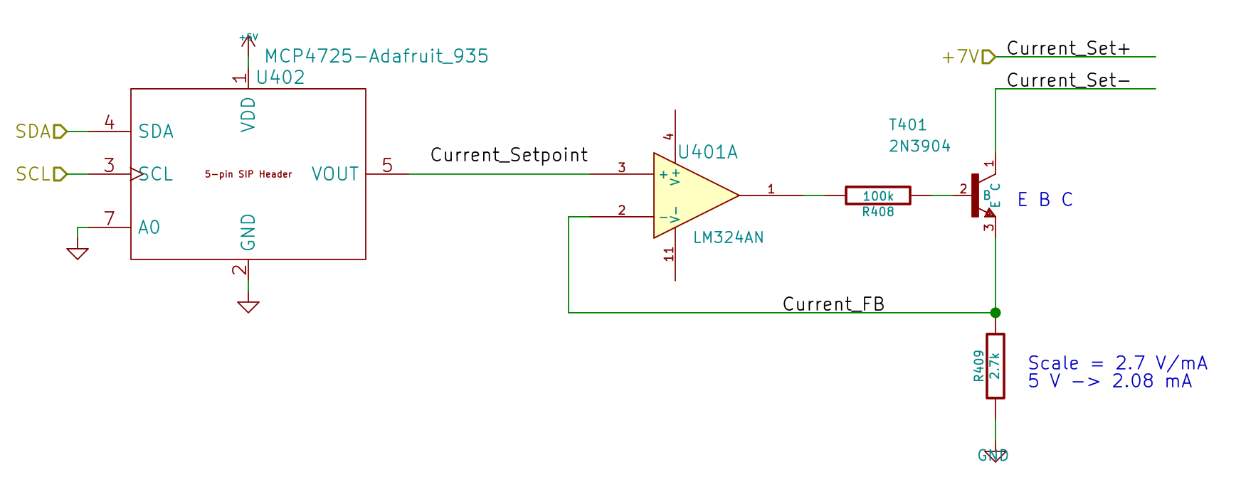
Because the motor will draw more current during pulsed operation, the ET227 needs more base drive. The existing circuit topped out around 2.5 A, so I reduced the current sampling resistor by a bit:

Optoisolator Driver

If you care about the exact current, you’d use a 1% resistor, but if you care about the current, you’ll be doing closed-loop feedback to compensate for the transistor gain variations. Compared to those, the resistor doesn’t matter.

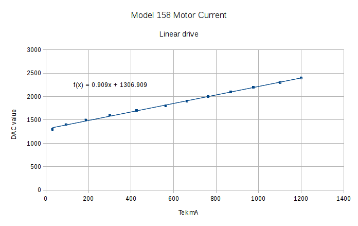
Running the MCP4725 DAC through its range produces a nice graph:

Current Calibrate – DAC – 270k Hall 2.7k opto

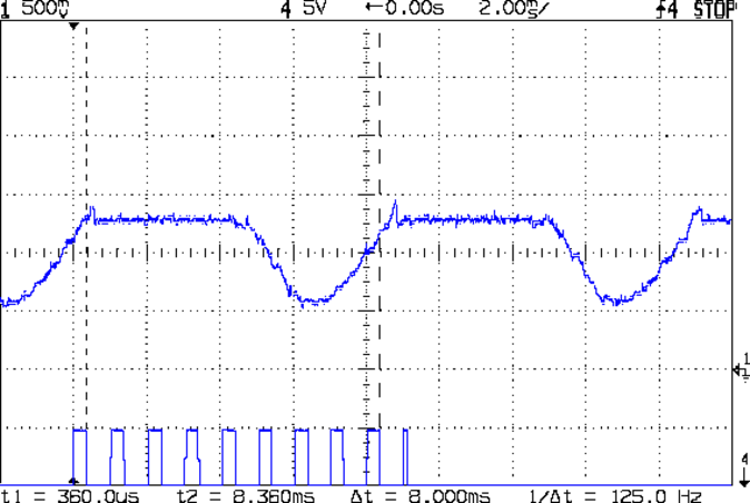
The X axis comes from the Tek Hall-effect current probe, so the numbers don’t depend on the ferrite toroid & differential amp calibration. They do, of course, require a bit of eyeballometric calibration to extract the flat top from the waveform, as shown by this old waveform:

Motor current – ADC sample timing

Ya gotta start somewhere.

The linear fit to those dots gives the DAC value required to produce the observed current, at least for these particular transistors at whatever temperature they’re at in a rather chilly Basement Laboratory.

Of course, the observed current tops out at 1.2 A: the motor’s peak current during normal linear operation. The line looks so pretty that I’ll assume it continues upward to the maximum 12-bit DAC value of 4095 and the corresponding ET227 current. Working backwards, that will be 3.1 A and should suffice for all but the highest peaks at high line voltage.

2014-12-26
Kenmore 158: Recalibrated Hall Effect Sensor Amp

Reducing the differential amp gain fits a higher current into the Arduino’s fixed 5 V ADC range:

Hall Sensor Differential Amp

Those are 1% resistors, chosen from the heap for being pretty close to what I needed. Given that it’s an LM324 op amp, we’re not talking instrumentation grade results here.

The same calibration run that produced the DAC plot gave these values:

Current Calibrate – ADC – 270k Hall 2.7k opto

The linear fit gives the actual current, as seen by the Tek probe, for a given ADC reading.

The trimpot controls the offset voltage at zero current; working backwards, ADC = 0 corresponds to 140 mV, a bit higher than the actual 90 mV. Close enough, at least for a linear fit to eyeballed data, sez I.

Working forward, the maximum ADC value of 1023 corresponds to 4 A, which should suffice.

2014-12-24
Kenmore 158: Pulse Drive
A Circuit Cellar reader sent me a lengthy note describing his approach to slow-motion AC motor drives, designed for an already ancient truck mounted radar antenna back in 1972-ish, that prompted me to try it his way.

The general idea is to pulse the motor at full current for half a power line cycle with an SCR (rather than a triac) at a variable pulse repetition rate: the high current pulse ensures that the motor will start turning and the variable repetition frequency determines the average speed. As he puts it, the motor will give off a distinct tick at very low speeds and the maximum speed will depend on how the motor reacts to half-wave drive.

Note that this is not the chopped-current approach to speed control: the SCR always begins conducting at the first positive-going 0 V crossing after the command and continues until the motor current drops to zero. There are no sharp edges generating high-pitched acoustic noise and EMI: silence is golden.

The existing speed control circuitry limits the peak current and assumes that the motor trundles along more-or-less steadily. That won’t be the case when it’s coasting between discontinuous current pulses.

When I first looked at running the motor on DC, these measurements showed the expected relationship:

Kenmore Model 158 AC Motor on DC – Loaded and Unloaded RPM vs Voltage

Later on, plotting RPM against current (50 mA/step starting at 550 mA):

Motor RPM vs Current Steps – Accelerating

Eyeballometrically, the slowest useful speed will be 2 stitch/s = 120 shaft RPM = 1300 motor RPM. At that speed, under minimal load, the motor runs on about 20 V and draws 550 mA. At that current, the 40 Ω winding drops 22 V, which we’ll define as “about 20 V” for this discussion, so the back EMF amounts to pretty nearly zilch.

That’s what you’d expect for the fraction of a second while the motor comes up to full speed, but in this case it never reaches full speed, so the motor current during the pulses will be limited only by the winding resistance. At the 200 V peak I’ve been using for the high-line condition, that’s about 5 A peak, although I’d expect 4 A to be more typical.

So, in order to make this work:
- the optocoupler driving the base needs more current
- the differential amp from the Hall effect sensor needs less gain
Given the ease with which I’ve pushed the hulking ET227 transistor out of its SOA, the motor definitely needs a flyback diode to direct the winding current away from the collector as the transistor shut off at the end of the pulse. Because it’s running from full-wave rectified AC, the winding current never drops to zero: there will definitely be enough current to wreck the transistor.

The firmware needs reworking to produce discrete pulses at a regular pace, rather than slowly adjusting the current over time, but that’s a simple matter of software…
2014-12-22

Kenmore 158: Current Sensor Calibration

The first task: produce an equation that converts raw ADC values into actual motor current. This is not quite the same as the DC calibration, because the motor current is neither clean nor stable.

Step the output current setpoint in 50 mA increments from 450 mA to 1100 mA and remain at each setpoint for 10 seconds while dumping measurements every 500 ms. The ADC count comes from the sampling / sorting / selection process that attempts to pick out either the not really flat top of the current-limited waveform or the peak of the non-limited sine wave.

Convert the raw data dump into a spreadsheet to get a block like this for each current setpoint:

Motor RPM	Shaft RPM	Setpoint mA	DAC count	ADC count	Noisy mA	Comp mA
Setpoint: 600	DACvalue: 2372
3797	334	600	2372	266	724	540
4465	399	600	2372	263	715	532
4734	416	600	2372	265	721	538
4834	438	600	2372	263	715	532
4829	433	600	2372	264	718	535
4857	438	600	2372	264	718	535
4900	438	600	2372	265	721	538
4859	436	600	2372	266	724	540
4887	445	600	2372	265	721	538
4926	446	600	2372	263	715	532
4884	438	600	2372	265	721	538
4890	442	600	2372	264	718	535
4913	440	600	2372	264	718	535
4866	436	600	2372	263	715	532
4895	434	600	2372	264	718	535
4890	442	600	2372	266	724	540
4884	438	600	2372	266	724	540
4913	442	600	2372	265	721	538
4913	441	600	2372	266	724	540
4878	436	600	2372	264	718	535
				265

The lone number on the bottom row is the computed average of the ADC counts for the block, which I did in the spreadsheet rather than in the firmware.

During each ten second interval, set the scope voltage cursor to the eyeballed “correct” value of the motor current waveform, as measured on the Tek current probe. There’s no way to automate this, because only the human eyeball can pick out the, ah, true current measurement amid all the clutter:

Calibrate - Hall amp - Tek 200 mA-div — Calibrate – Hall amp – Tek 200 mA-div

For each current setpoint value, create a line with the manually measured true voltage from the scope trace, the calculated true current (using the Tek probe’s front panel scale), along with the DAC setpoint and the average ADC values extracted from each block of that giant data dump:

Setpoint mA	Scope mV	Actual mA	DAC count	ADC count
450	21.80	436	2205	197
500	25.94	519	2261	225
550	29.06	581	2316	245
600	31.56	631	2372	265
650	34.38	688	2427	285
700	36.88	738	2483	304
750	39.69	794	2538	324
800	42.19	844	2594	340
850	45.00	900	2649	350
900	47.50	950	2705	361
850	46.86	937	2649	356
800	43.75	875	2594	348
750	41.25	825	2538	335
700	39.06	781	2483	318
650	36.56	731	2427	302
600	34.38	688	2372	285
550	32.50	650	2316	270
500	30.31	606	2261	253
450	27.81	556	2205	237
400	25.63	513	2150	220

Plot each actual motor current against the corresponding average ADC value:

The linear fit breaks down toward 1 A, because measuring the actual peak of a noisy sine wave doesn’t work well, but the values aren’t all that far off.

Given an ADC value, that equation converts it directly into the actual motor current as estimated by the human eyeball, taking into account all the measurement weirdness. The Hall sensor produces a voltage that’s linearly related to the current, so the reasonable linearity of the data says that the sampling / sorting / selection process actually produces pretty nearly the correct result across the entire operating current range.

Note that the equation doesn’t depend on the DAC output calibration; the ADC and Tek probe simply measure whatever current happens to pass through the motor for that DAC value. The current through the ET227 transistor doesn’t seem to change over the ten seconds required to take the manual measurement, so it’s all good.

2014-11-14

Tag: Arduino

Adafruit TFT LCD: Color Indicator Spots

Adafruit TFT Shield: Firmware Heartbeat Spot

Kenmore 158 UI: Automatic Button Builder

Kenmore 158: Recalibrated Optoisolator Drive

Kenmore 158: Recalibrated Hall Effect Sensor Amp

Kenmore 158: Pulse Drive

Kenmore 158: Current Sensor Calibration