Ed Nisley's Blog: Shop notes, electronics, firmware, machinery, 3D printing, laser cuttery, and curiosities. Contents: 100% human thinking, 0% AI slop.
Category: Software
General-purpose computers doing something specific
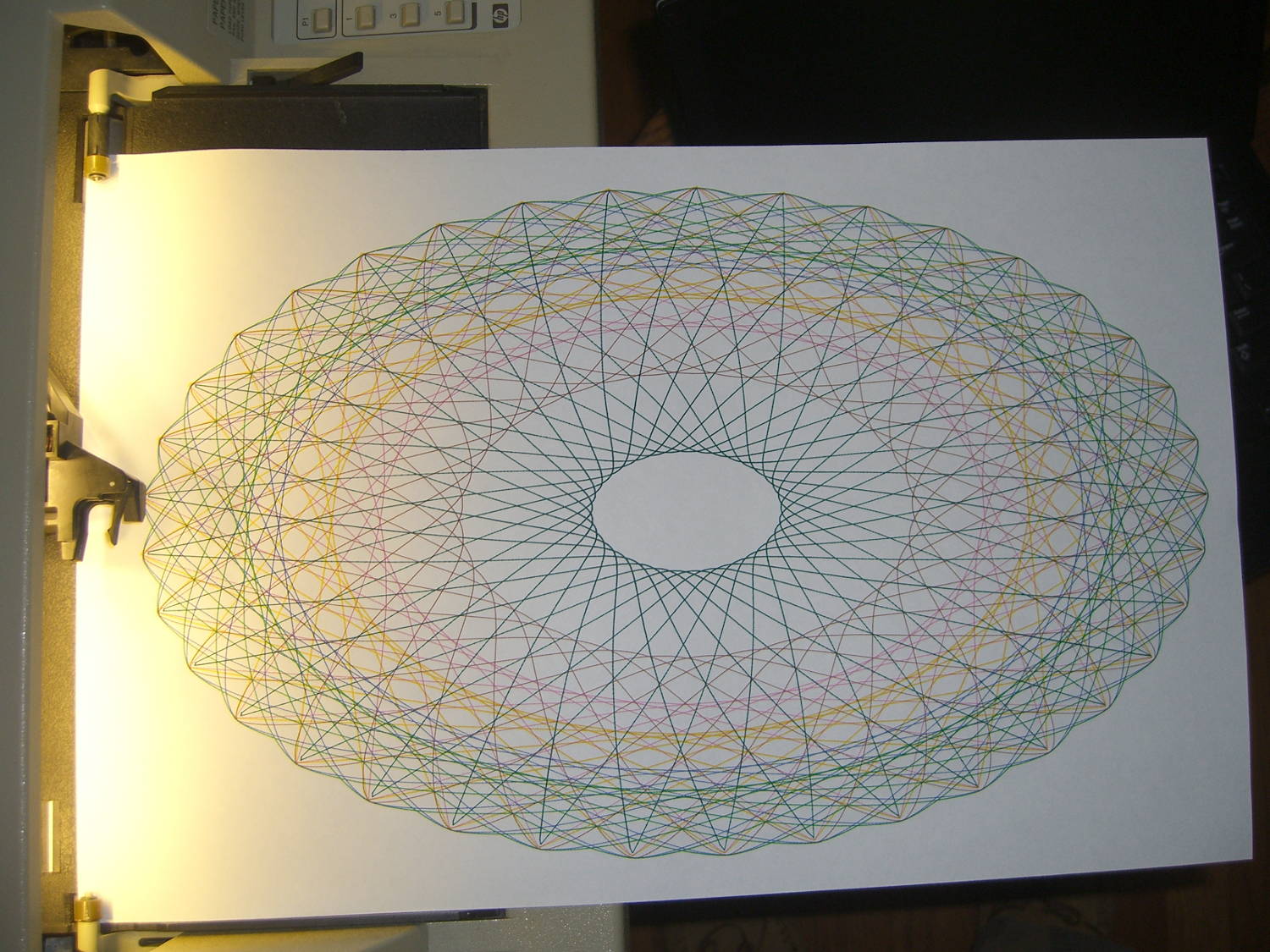
Setting n2=n3=1.5 generates smoothly rounded shapes, rather than the spiky ones produced by n2=n3=1.0, so I combined the two into a single demo routine:
HP 7475A – SuperFormula patterns
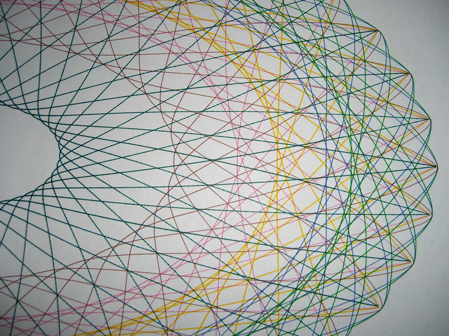
A closer look shows all the curves meet at the points, of which there are 37:
HP 7475A – SuperFormula patterns – detail
The spikes suffer from limited resolution: each curve has 10 k points, but if the extreme end of a spike lies between two points, then it gets blunted on the page. Doubling the number of points would help, although I think this has already gone well beyond the, ah, point of diminishing returns.
I used the three remaining “disposable” liquid ink pens for the spiked curves; the black pen was beyond repair. They produce gorgeous lines, although the magenta ink seems a bit thinned out by the water I used to rinse the remains of the last refill out of the spiral vent channel.
I modified the Chiplotle supershape() function to default to my choices for point_count and travel, then copied the superformula() function and changed it to return polar coordinates, because I’ll eventually try scaling the linear value as a function of the total angle, which is much easier in polar coordinates.
The demo code produces the patterns in the picture by iterating over interesting values of n1 and n2=n3, stepping through the pen carousel for each pattern. As before, m should be prime/10 to produce a prime number of spikes / bumps. You could add more iteration values, but six of ’em seem entirely sufficient.
A real demo should include a large collection of known-good parameter sets, from which it can pick six sets to make a plot. A legend documenting the parameters for each pattern, plus the date & time, would bolster the geek cred.
The Python source code with the modified Chiplotle routines:
from chiplotle import *
from math import *

def superformula_polar(a, b, m, n1, n2, n3, phi):
   ''' Computes the position of the point on a
   superformula curve.
   Superformula has first been proposed by Johan Gielis
   and is a generalization of superellipse.
   see: http://en.wikipedia.org/wiki/Superformula
   Tweaked to return polar coordinates
   '''

   t1 = cos(m * phi / 4.0) / a
   t1 = abs(t1)
   t1 = pow(t1, n2)

   t2 = sin(m * phi / 4.0) / b
   t2 = abs(t2)
   t2 = pow(t2, n3)

   t3 = -1 / float(n1)
   r = pow(t1 + t2, t3)
   if abs(r) == 0:
      return (0,0)
   else:
 #     return (r * cos(phi), r * sin(phi))
     return (r,phi)

def supershape(width, height, m, n1, n2, n3,
   point_count=10*1000, percentage=1.0, a=1.0, b=1.0, travel=None):
   '''Supershape, generated using the superformula first proposed
   by Johan Gielis.

   - `points_count` is the total number of points to compute.
   - `travel` is the length of the outline drawn in radians.
      3.1416 * 2 is a complete cycle.
   '''
   travel = travel or (10*2*pi)

   ## compute points...
   phis = [i * travel / point_count
      for i in range(1 + int(point_count * percentage))]
   points = [superformula_polar(a, b, m, n1, n2, n3, x) for x in phis]

   ## scale and transpose...
   path = [ ]
   for r, a in points:
      x = width * r * cos(a)
      y = height * r * sin(a)
      path.append(Coordinate(x, y))

   return Path(path)

## RUN DEMO CODE

if __name__ == '__main__':
   paperx = 8000
   papery = 5000
   if  not False:
     plt=instantiate_plotters()[0]
     plt.set_origin_center()
     plt.write(hpgl.VS(10))
     pen = 1
     for m in [3.7]:
        for n1 in [0.20, 0.60, 0.8]:
          for n2 in [1.0, 1.5]:
              n3 = n2
              e = supershape(paperx, papery, m, n1, n2, n3)
              plt.select_pen(pen)
              if pen < 6:
                 pen += 1
              else:
                 pen = 1
              plt.write(e)
     plt.select_pen(0)
   else:
     e = supershape(paperx, papery, 1.9, 0.8, 3, 3)
     io.view(e)
Although the Superformula can produce a bewildering variety of patterns, I wanted to build an automated demo that plotted interesting sets of similar results. Herewith, some notes after an evening of fiddling around with the machinery.
The first two parameters set the more-or-less maximum X and Y values in plotter units; the plot is centered at zero and will extend that far in both the positive and negative directions. For US paper:
A = Letter = 11 x 8½ inch → 4900 x 3900
B = 17 x 11 inch → 8000 x 5000
The point_count parameter defines the number of points to be plotted for the entire figure. They’re uniformly distributed in angle, not in distance, so some parts of the figure will plot very densely and others sparsely, but the plotter will connect all of the points with straight lines and it’ll look reasonably OK. For the figures below, 10*1000 works well.
The travel value defines the number of full cycles that the figure will make, in units of 2π. Ten cycles seems about right.
The four parameters in between those are the m, n1, n2, and n3 values plugged directly into the basic Superformula. The latter two are exponents of the trig terms; 1.0 seems less bizarre than anything else.
Sooo, that leaves only two knobs…
With travel set for 10 full cycles, m works best when set to a value that’s equal to prime/10, which produces prime points around the figure. Thus, if you want 11 points, use m=1.1 and for 51 points, use m=5.1. Some non-prime numbers produce useful patterns (as below), others collapse into just a few points.
The n1 parameter is an overall exponent for the whole formula in the form -1/n1. Increasing values, from 0.1 to about 2.0, expand the innermost points of the pattern outward and turn the figure into more of a ring and less of a lattice.
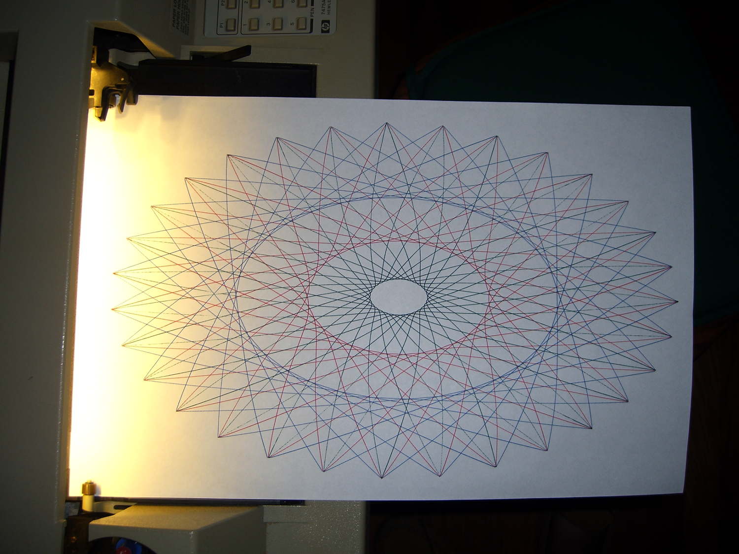
So, for example, with m=3.1, setting n1= 0.15, 0.30, 0.60 produces this pattern with 31 points:
HP 7475A – Superformula – m 3.1 vary n1
Varying both at once, thusly: (m,n1) = (1.9,0.20)=green (3.7,0.30)=red (4.9,0.40)=blue
produces this pattern:
HP 7475A – Superformula – m 1.9 3.7 4.9 n1 0.2 0.3 0.4
Yeah, 49 isn’t a prime number. It’s interesting, though.
Note that n1 doesn’t set the absolute location of the innermost points; you must see how it interacts with m before leaping to any conclusions.
It’s still not much in the way of Art, but it does keep the plotter chugging along for quite a while and that’s the whole point. I must yank the functions out of the Chiplotle library, set my default values, add one point to automagically close the last vertex, and maybe convert them to polar coordinates to adjust the magnitude as a function of angle.
Yes, that poor green ceramic-tip pen is running out of ink after all these decades.
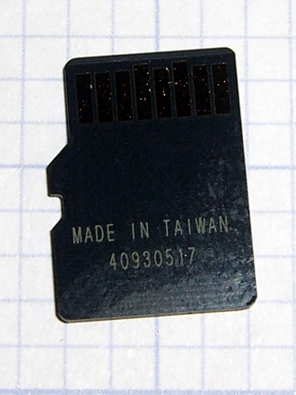
The previous cards were made in Korea, but this one came from Taiwan with a different serial number format:
Sony SR-64UX 64 GB MicroSDXC card – back
The tiny letters on the front identify it as an SR-64UX, but I haven’t been able to find any definitive Sony source describing the various cards; their catalog page listing cards for digital still cameras may be as good as it gets. This one seems to have a higher read speed, for whatever little good that may do.
It stored and regurgitated the usual deluge of video files with no problem, which is only to be expected. This time around, I checked the MD5 sums, rather than unleashing diff on the huge files:
cd /media/ed/9C33-6BBD/
for f in * ; do find /mnt/video/ -name $f | xargs md5sum $f ; done
11e31c9ba3befbef6dd3630bb68064d6 MAH00539.MP4
11e31c9ba3befbef6dd3630bb68064d6 /mnt/video/2015-07-05/MAH00539.MP4
... snippage ...
It now sits in the fancy plastic display case that the HDR-AS30V camera came in until the previous replacement card fails.
Verily, ImageMagick can do nearly anything you want to an image, as long as you know how to ask for it:
for f in *png ; do convert $f -density 300 -define jpeg:extent=200KB ${f%%.*}.jpg ; done
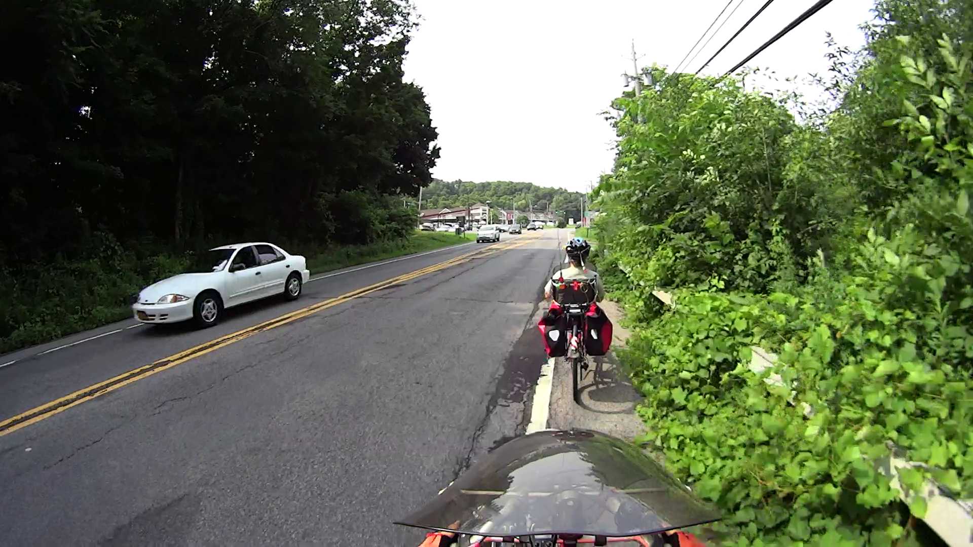
That converts a directory full of VLC’s video snapshot images from PNG format, which require nigh onto 4 MB each, into correspondingly named JPG files under 200 kB. The image quality may not be the greatest, but it’s good enough to document road hazards in emails.
Rt 376 2015-07-06 – Walker to Maloney – 3
The density option overrides VLC’s default 72 dpi, which doesn’t matter until a program attempts to show the image at “actual size”.
I didn’t realize that the define option existed, but it seems to be how you jam specific controls into the various image coders & decoders. Some of the “artifacts”, well, I can’t even pronounce…
VLC’s snapshot file names look like vlcsnap-2015-07-06-12h10m27s10.png, so bulk renaming and resequencing will be in order.
Although I’d thought of a Mu-metal shield, copper foil tape should be easier and safer to shape into a simple shield. The general idea is to line the interior with copper tape, solder the joints together, cover with Kapton tape to reduce the likelihood of shorts, then stick it in place with some connector pin-and-socket combinations. Putting the tape on the outside would be much easier, but that would surround the circuitry with a layer of plastic that probably carries enough charge to throw things off.
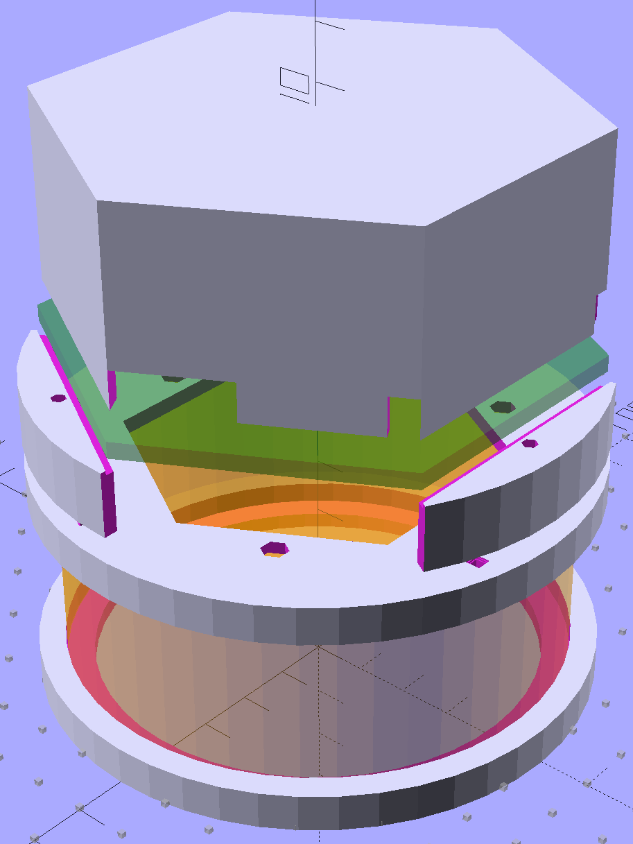
Anyhow, the hexagonal circuit board model now sports a hexagonal cap to support the shield:
Victoreen 710-104 Ionization Chamber Fittings – Show with shield
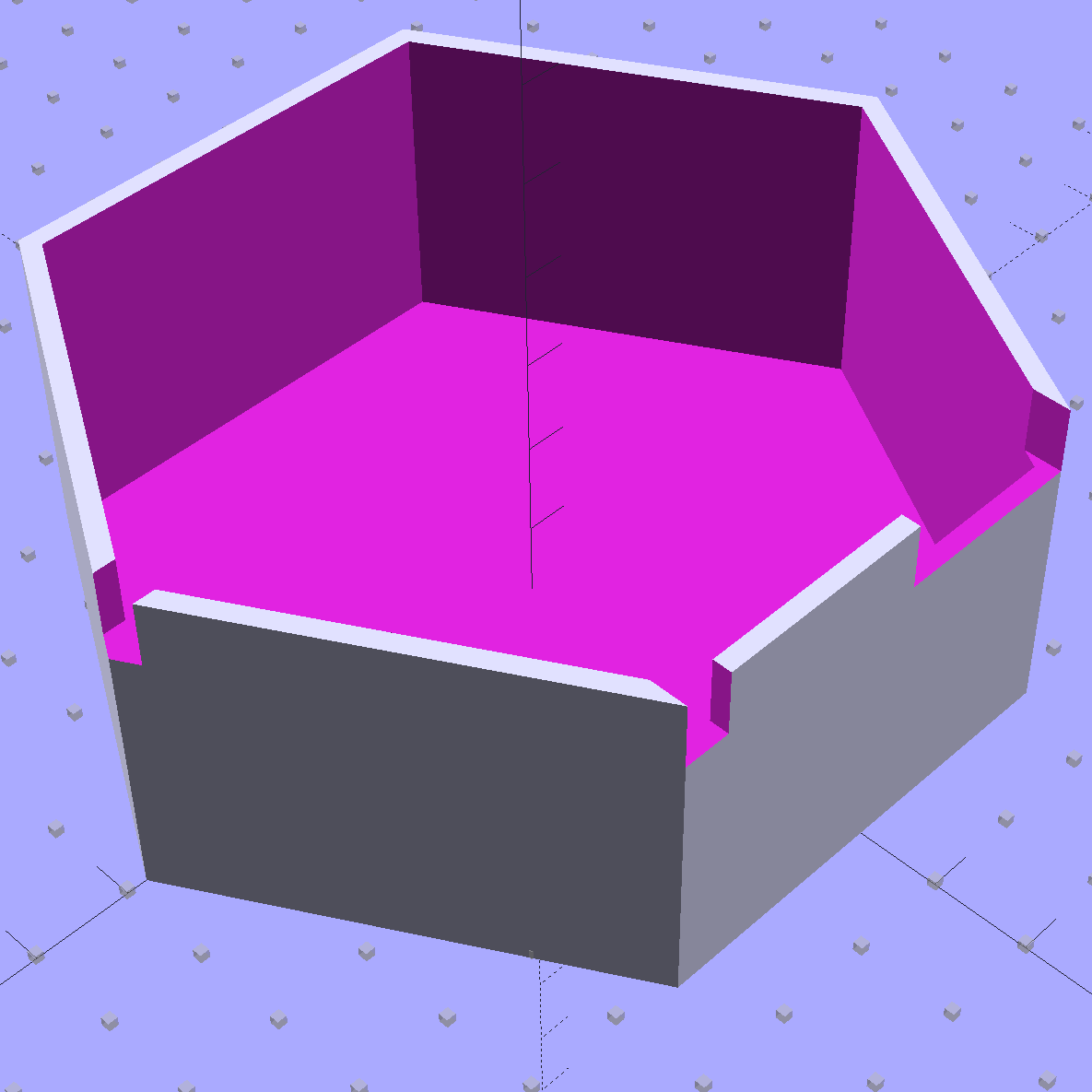
The ad-hoc openings fit various switches, wires, & twiddlepots:
The general idea is to put the electrometer circuitry directly atop the Victoreen 710-104 ionization chamber, so as to minimize the distance from the center collector electrode to the electrometer input. After a few false starts, this looked promising:
Victoreen 710-104 Ionization Chamber Fittings – Show layout
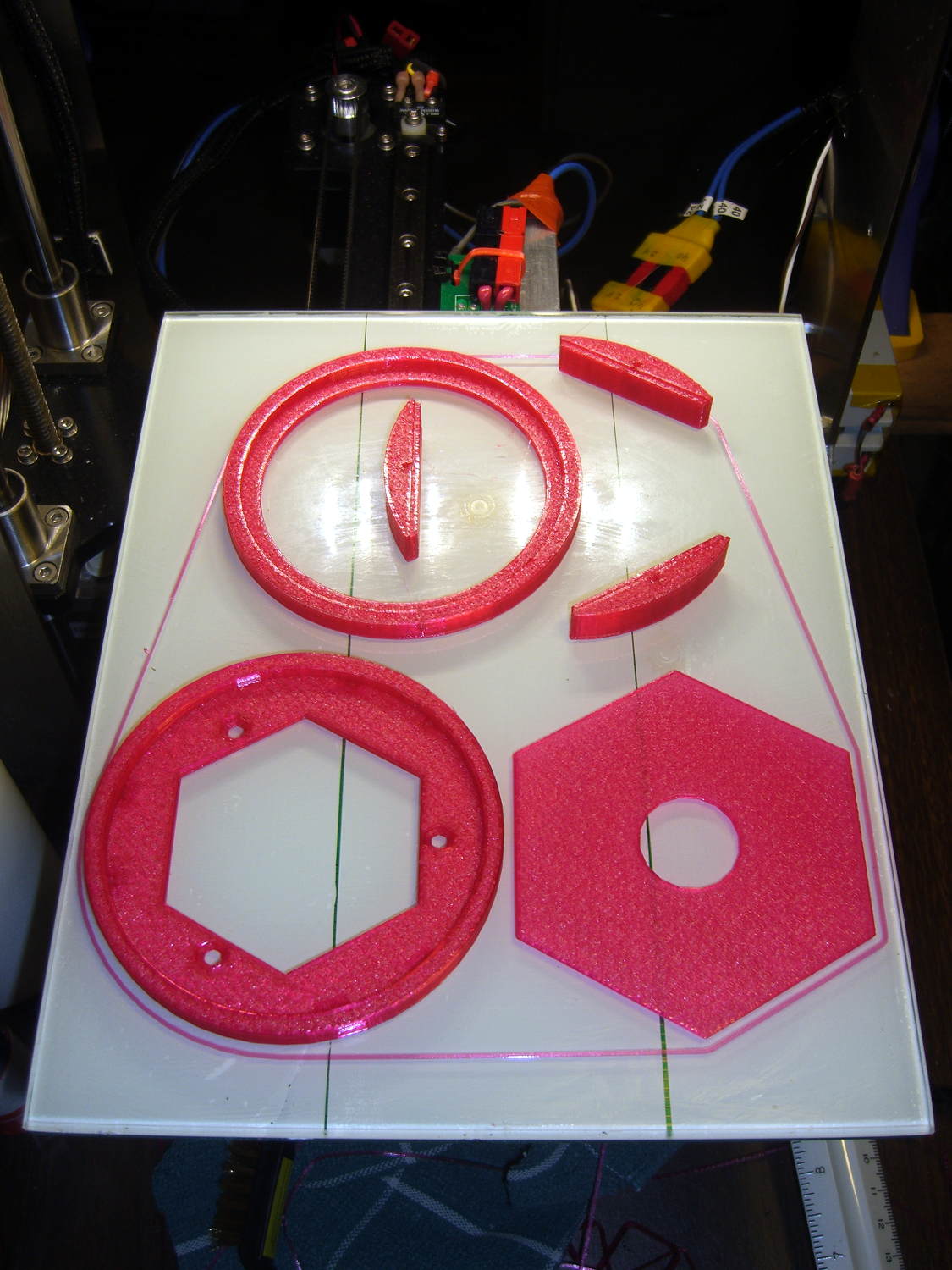
The hexagonal circuit board fits the can so nicely that I’ll run with it, despite the over-the-top twee factor. Because it’s so hard to freehand a hex, I printed the green object as a tracing template, despite having the Slic3r preview show the parts just barely fitting on the M2 platform:
The skirt measures 0.25±0.05 around the entire perimeter, with a slight positive bias (platform too low) along the left side and a corresponding negative bias on the right. Both sides look just fine to me.
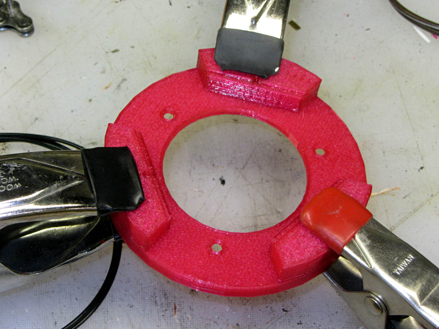
A pair of alignment pegs hold each board support in place while gluing:
Victoreen 710-104 Fittings – clamping
Next time around, I’ll glue the supports with the circuit board template laid in place to ensure the edges have the proper orientation, but they came out surprisingly close just by matching the outer perimeters. Of course, I probably bandsawed / belt sanded the carefully traced hex just slightly off-kilter.
The outer perimeter has 48 sides. Making it a multiple of three means each board support has the same pattern of sides and all will be interchangeable. Making it a multiple of four means each quadrant has the same pattern of sides and the ring looks pleasingly symmetrical. The factor-of-three is most important: you want interchangeable supports. Trust me on this.
The bottom ring keeps the solder dimple that seals the can base off the desk, but I also stuck a quartet of rubber feet on the can for better traction.
Here’s what it looks like with the two A23 12 V bias batteries in their holders, affixed to the can with foam tape:
Victoreen 710-104 Fittings – assembled
The OpenSCAD source code includes a few more tweaks:
// Victoreen 710-104 Ionization Chamber Fittings
// Ed Nisley KE4ZNU July 2015

Layout = "Show";
					// Show - assembled parts
					// Build - print them out!
					// CanCap - PCB insulator for 6-32 mounting studs
					// CanBase - surrounding foot for ionization chamber
					// CanLid - generic surround for either end of chamber
					// PCB - template for cutting PCB sheet
					// PCBBase - holder for PCB atop CanCap

BuildTemplate = false;			// true to build PCB template along with everything else

//- Extrusion parameters must match reality!
//  Print with 2 shells and 3 solid layers

ThreadThick = 0.25;
ThreadWidth = 0.40;

HoleWindage = 0.2;

Protrusion = 0.1;			// make holes end cleanly

AlignPinOD = 1.75;			// assembly alignment pins = filament dia

inch = 25.4;

function IntegerMultiple(Size,Unit) = Unit * ceil(Size / Unit);

//- Screw sizes

Tap4_40 = 0.089 * inch;
Clear4_40 = 0.110 * inch;
Head4_40 = 0.211 * inch;
Head4_40Thick = 0.065 * inch;
Nut4_40Dia = 0.228 * inch;
Nut4_40Thick = 0.086 * inch;
Washer4_40OD = 0.270 * inch;
Washer4_40ID = 0.123 * inch;


//----------------------
// Dimensions

OD = 0;											// name the subscripts
LENGTH = 1;

Chamber = [91.0 + HoleWindage,38];				// Victoreen ionization chamber dimensions

Stud = [										// stud welded to ionization chamber lid
	[6.5,IntegerMultiple(0.8,ThreadThick)],		// flat head -- generous clearance
	[4.0,9.5],									// 6-32 screw -- ditto
];
NumStuds = 3;
StudSides = 6;									// for hole around stud

BCD = 2.75 * inch;								// mounting stud bolt circle diameter

PlateThick = 3.0;								// layer atop and below chamber ends
RimHeight = 4.0;								// extending up along chamber perimeter
WallHeight = RimHeight + PlateThick;
WallThick = 5.0;								// thick enough to be sturdy & printable
CapSides = 8*6;									// must be multiple of 4 & 3 to make symmetries work out right

PCBFlatsOD = 85.0 + 2*ThreadWidth;				// hex dia across flats + clearance
PCBThick = 1.1;
PCB = [PCBFlatsOD / cos(30),PCBThick - ThreadThick];		// OD = tip-to-tip dia

echo(str("Actual PCB across flats: ",PCBFlatsOD - 2*ThreadWidth));
echo(str(" ... tip-to-tip dia: ",(PCBFlatsOD - 2*ThreadWidth)/cos(30)));
echo(str(" ... thickness: ",PCBThick));

HolderHeight = 11.0 + PCB[LENGTH];				// thick enough for PCB to clear studs
HolderShelf = 2.0;								// shelf under PCB edge

echo(str("PCB holder height: ",HolderHeight));
echo(str(" ... across flats: ",PCBFlatsOD));

//----------------------
// Useful routines

module PolyCyl(Dia,Height,ForceSides=0) {			// based on nophead's polyholes

  Sides = (ForceSides != 0) ? ForceSides : (ceil(Dia) + 2);

  FixDia = Dia / cos(180/Sides);

  cylinder(r=(FixDia + HoleWindage)/2,
           h=Height,
	   $fn=Sides);
}

//- Locating pin hole with glue recess
//  Default length is two pin diameters on each side of the split

module LocatingPin(Dia=AlignPinOD,Len=0.0) {

	PinLen = (Len != 0.0) ? Len : (4*Dia);

	translate([0,0,-ThreadThick])
		PolyCyl((Dia + 2*ThreadWidth),2*ThreadThick,4);

	translate([0,0,-2*ThreadThick])
		PolyCyl((Dia + 1*ThreadWidth),4*ThreadThick,4);

	translate([0,0,-Len/2])
		PolyCyl(Dia,Len,4);

}

module ShowPegGrid(Space = 10.0,Size = 1.0) {

  RangeX = floor(100 / Space);
  RangeY = floor(125 / Space);

	for (x=[-RangeX:RangeX])
	  for (y=[-RangeY:RangeY])
		translate([x*Space,y*Space,Size/2])
		  %cube(Size,center=true);
}

//-----

module CanLid() {

	difference() {
		cylinder(d=Chamber[OD] + 2*WallThick,h=WallHeight,$fn=CapSides);
		translate([0,0,PlateThick])
			PolyCyl(Chamber[OD],Chamber[1],CapSides);
	}

}

module CanCap() {

	difference() {
		CanLid();

		translate([0,0,-Protrusion])											// central cutout
//			cylinder(d=(BCD - 2*5.0),h=Chamber[LENGTH],$fn=CapSides);
			rotate(180/6)
				cylinder(d=BCD,h=Chamber[LENGTH],$fn=6);

		for (i=[0:(NumStuds - 1)])												// stud clearance holes
			rotate(i*360/NumStuds)
				translate([BCD/2,0,0])
					rotate(180/StudSides) {
						translate([0,0,(PlateThick - (Stud[0][LENGTH] + 2*ThreadThick))])
							PolyCyl(Stud[0][OD],2*Stud[0][LENGTH],StudSides);
						translate([0,0,-Protrusion])
							PolyCyl(Stud[1][OD],2*Stud[1][LENGTH],StudSides);
					}

		for (i=[0:(NumStuds - 1)], j=[-1,1])									// PCB holder alignment pins
			rotate(i*360/NumStuds + j*15 + 60)
				translate([Chamber[OD]/2,0,0])
					rotate(180/4)
						LocatingPin(Len=2*PlateThick - 2*ThreadThick);
	}

}

module CanBase() {

	difference() {
		CanLid();
		translate([0,0,-Protrusion])
			PolyCyl(Chamber[OD] - 2*5.0,Chamber[1],CapSides);
	}
}

module PCBTemplate() {

	difference() {
		cylinder(d=((PCBFlatsOD - 2*ThreadWidth)/cos(30)),h=max(PCB[LENGTH],3.0),$fn=6);		// actual PCB size, overly thick
		translate([0,0,-Protrusion])
			cylinder(d=10,h=10*PCB[LENGTH],$fn=12);
	}
}

module PCBBase() {

	difference() {
		cylinder(d=Chamber[OD] + 2*WallThick,h=HolderHeight,$fn=CapSides);

		rotate(30) {
			translate([0,0,-Protrusion])										// central hex
				cylinder(d=(PCBFlatsOD - 2*HolderShelf)/cos(30),h=2*HolderHeight,$fn=6);

			translate([0,0,HolderHeight - PCB[LENGTH]])							// hex PCB recess
				cylinder(d=PCB[OD],h=HolderHeight,$fn=6);

			for (i=[0:NumStuds - 1])											// PCB retaining screws
				rotate(i*120 + 30)
					translate([(PCBFlatsOD/2 + Clear4_40/2 + ThreadWidth),0,-Protrusion])
						rotate(180/6)
							PolyCyl(Tap4_40,2*HolderHeight,6);

			for (i=[0:(NumStuds - 1)], j=[-1,1])								// PCB holder alignment pins
				rotate(i*360/NumStuds + j*15 + 30)
					translate([Chamber[OD]/2,0,0])
						rotate(180/4)
							LocatingPin(Len=PlateThick);
		}

		for (i=[0:NumStuds - 1])												// segment isolation
			rotate(i*120 - 30)
				translate([0,0,-Protrusion]) {
					linear_extrude(height=2*HolderHeight)
						polygon([[0,0],[Chamber[OD],0],[Chamber[OD]*cos(60),Chamber[OD]*sin(60)]]);
				}
	}


}


//----------------------
// Build it

ShowPegGrid();

if (Layout == "CanLid") {
	CanLid();
}

if (Layout == "CanCap") {
	CanCap();
}

if (Layout == "CanBase") {
	CanBase();
}

if (Layout == "PCBBase") {
	PCBBase();
}

if (Layout == "PCB") {
	PCBTemplate();
}

if (Layout == "Show") {
	CanBase();
	color("Orange",0.5)
		translate([0,0,PlateThick + Protrusion])
			cylinder(d=Chamber[OD],h=Chamber[LENGTH],$fn=CapSides);
	translate([0,0,(2*PlateThick + Chamber[LENGTH] + 2*Protrusion)])
		rotate([180,0,0])
			CanCap();
	translate([0,0,(2*PlateThick + Chamber[LENGTH] + 5.0)])
		PCBBase();
	color("Green",0.5)
		translate([0,0,(2*PlateThick + Chamber[LENGTH] + 7.0 + HolderHeight)])
			rotate(30)
				PCBTemplate();
}

if (Layout == "Build") {

	if (BuildTemplate) {
		translate([-0.50*Chamber[OD],-0.60*Chamber[OD],0])
			CanCap();

		translate([0.55*Chamber[OD],-0.60*Chamber[OD],0])
			rotate(30)
				PCBTemplate();
	}
	else {
		translate([-0.25*Chamber[OD],-0.60*Chamber[OD],0])
			CanCap();
	}

	translate([-0.25*Chamber[OD],0.60*Chamber[OD],0])
		CanBase();
	translate([0.25*Chamber[OD],0.60*Chamber[OD],0])
		PCBBase();
}
Given Cycliq’s tech support recommendation to never, ever delete files from the camera’s MicroSD card, I’m now copying the files to the 500 GB network drive thusly:
rsync -au --progress /media/ed/Fly6 /mnt/video/
The Fly6 saws off a 400-800 MB file every 10.000 minutes, so a typical ride produces 4 GB of data.
The Sony HDR-AS30V emits a 4.2 GB file every 22:43 minutes: call it 12 GB per ride.
Somewhat to my surprise, both copy operations can proceed concurrently at 4 MB/s apiece. For unknown reasons, the drive doesn’t record the creation times for any data files:
ll /mnt/video/Fly6/DCIM/10450608/
total 4.2G
-rwxr-xr-x 1 ed root 476M 2057-09-06 19:40 14350001.AVI
-rwxr-xr-x 1 ed root 559M 2057-09-06 19:40 14450002.AVI
-rwxr-xr-x 1 ed root 568M 2057-09-06 19:40 14550003.AVI
-rwxr-xr-x 1 ed root 559M 2057-09-06 19:40 15040004.AVI
-rwxr-xr-x 1 ed root 277M 2057-09-06 19:40 15140005.AVI
-rwxr-xr-x 1 ed root 476M 2057-09-06 19:40 15240006.AVI
-rwxr-xr-x 1 ed root 476M 2057-09-06 19:40 15340007.AVI
-rwxr-xr-x 1 ed root 476M 2057-09-06 19:40 15440008.AVI
-rwxr-xr-x 1 ed root 424M 2057-09-06 19:40 15540009.AVI
The directories generally have the right dates, though, so maybe I’ve screwed up an obscure Samba / CIFS settings. The diratime option should be turned on by default.