Ed Nisley's Blog: Shop notes, electronics, firmware, machinery, 3D printing, laser cuttery, and curiosities. Contents: 100% human thinking, 0% AI slop.
Category: Science
If you measure something often enough, it becomes science
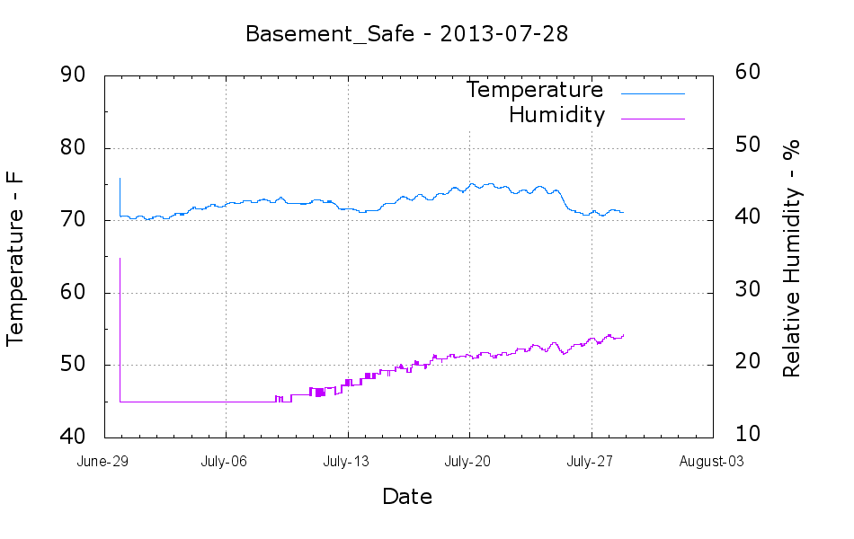
The humidity in the basement safe started rising this month:
Basement Safe – 2013-07-28
The bag of new silica gel weighed 575 g, so it adsorbed about 67 g of water as the humidity rose from bone dry to 24%. Last month it had soaked up 31 g, so the safe admits nearly an ounce of water each month with 50% RH in the basement. It takes five months to accumulate 60-ish g of water during the winter.
According to the Sorbent Systems charts, silica gel’s equilibrium capacity at 24% is about 12% of the gel’s weight, which would work out to 60 g. That’s close enough, methinks, given the graph resolution; the humidity changes slowly enough that it’s sorta-kinda equilibrated in there… 67 g works out to 13.4% of the dry weight, which is in the same ballpark.
I made up three more bags of dry gel (500 g + 7 or 8 g tare), tossed one in the safe, one in the 6 gallon plastic bucket of 3D printer filament, and one in an empty 6 gallon bucket for comparison. Some 6 dot (10-through-60%) humidity indicator cards are on their way, seeing as how I don’t have nearly enough dataloggers to keep up with the demand…
I put the XY coordinate origin in the middle of the platform, so that laying objects out for printing doesn’t require knowing how large the platform will be: as long as the printer is Big Enough, you (well, I) can print without further attention.
The RepRap world puts the XY coordinate origin in the front left corner of the platform, so that the platform size sets the maximum printable coordinates and all printing happens in Quadrant I. This has the (major, to some folks) advantage of using only positive coordinates, while requiring an offset for each different platform.
Yes, depending on which printer software you use, you can (automagically) center objects on your platform; this is often the only way to find objects created with Trimble (formerly Google) Sketchup. I am a huge fan of knowing exactly what’s going to happen before the printing starts, so I position my solid models exactly where I want them, right from the start. For example, this OpenSCAD model of the bike helmet mirror parts laid out for printing:
Helmet mirror mount – 3D model – Show layout
… exactly matches the plastic on the Thing-O-Matic’s platform, with the XY origin right down the middle of the platform:
Helmet mirror mount on build platform – smaller mirror shaft
It’d print exactly the same, albeit with more space around the edges, on the M2’s platform.
Similarly, the Z axis origin sits exactly on the surface of the platform. That way, the Z axis coordinate equals the actual height of the current thread extrusion in a measurable way: when you set the Z axis to, say, 2.0 mm, you can measure that exact distance between the extruder nozzle and the platform:
Taper gauge below nozzle
Now, admittedly, I fine-tune that distance by measuring the height of the skirt thread around the printed object, but the principle remains: a thread printed on the platform with Z=0.25 should be exactly 0.25 mm thick.
The start.gcode file handles all that:
;-- Slic3r Start G-Code for M2 starts --
;  Ed Nisley KE4NZU - 15 April 2013
M140 S[first_layer_bed_temperature]	; start bed heating
G90				; absolute coordinates
G21				; millimeters
M83				; relative extrusion distance
M84				; disable stepper current
G4 S3			; allow Z stage to freefall to the floor
G28 X0			; home X
G92 X-95			; set origin to 0 = center of plate
G1 X0 F30000		; origin = clear clamps on Y
G28 Y0			; home Y
G92 Y-127 		; set origin to 0 = center of plate
G1 Y-125 F30000	; set up for prime at front edge
G28 Z0			; home Z
G92 Z1.0			; set origin to measured z offset
M190 S[first_layer_bed_temperature]	; wait for bed to finish heating
M109 S[first_layer_temperature]	; set extruder temperature and wait
G1 Z0.0 F2000		; plug extruder on plate
G1 E10 F300		; prime to get pressure
G1 Z5 F2000		; rise above blob
G1 X5 Y-122 F30000	; move away from blob
G1 Z0.0 F2000		; dab nozzle to remove outer snot
G4 P1			; pause to clear
G1 Z0.5 F2000		; clear bed for travel
;-- Slic3r Start G-Code ends --
The wipe sequence, down near the bottom, positions the extruder at the front center edge of the glass plate, waits for it to reach the extrusion temperature, then extrudes 10 mm of filament to build up pressure behind the nozzle. The blob generally hangs over the edge of the platform and usually doesn’t follow the nozzle during the next short move and dab to clear the mess:
M2 – Wipe blobs on glass platform
I’ve also configured Slic3r to extrude at least 25 mm of filament in at least three passes around the object. After that, the extruder pressure has stabilized and the first layer of the object begins properly.
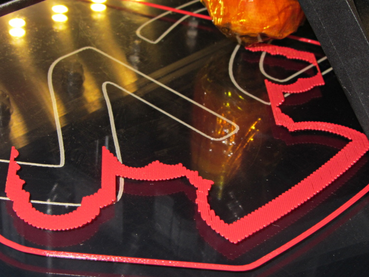
Which brings up another difference: the first layer printed on the platform is exactly like all the others. It’s not smooshed to get better adhesion or overfilled to make the threads stick together:
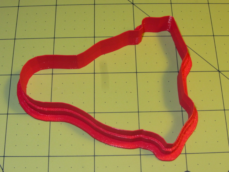
Robot cookie cutter – printing first layer
I print the first layer at 25 mm/s to give the plastic time to bond to the platform and use hairspray to make PLA stick to glass like it’s glued down.
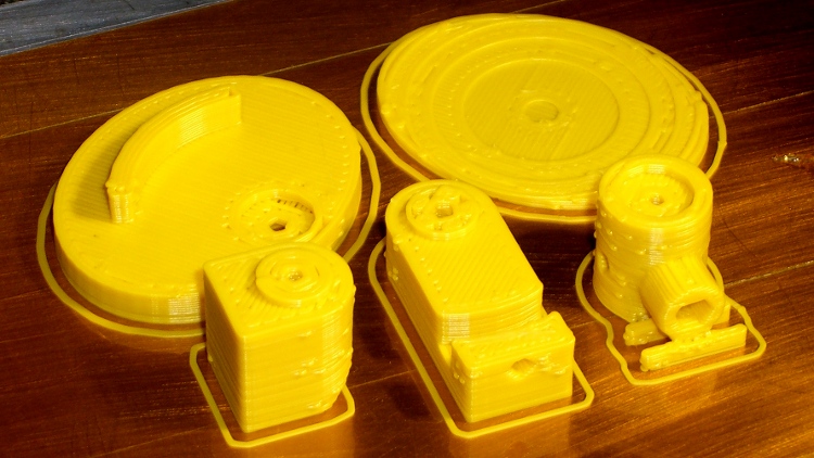
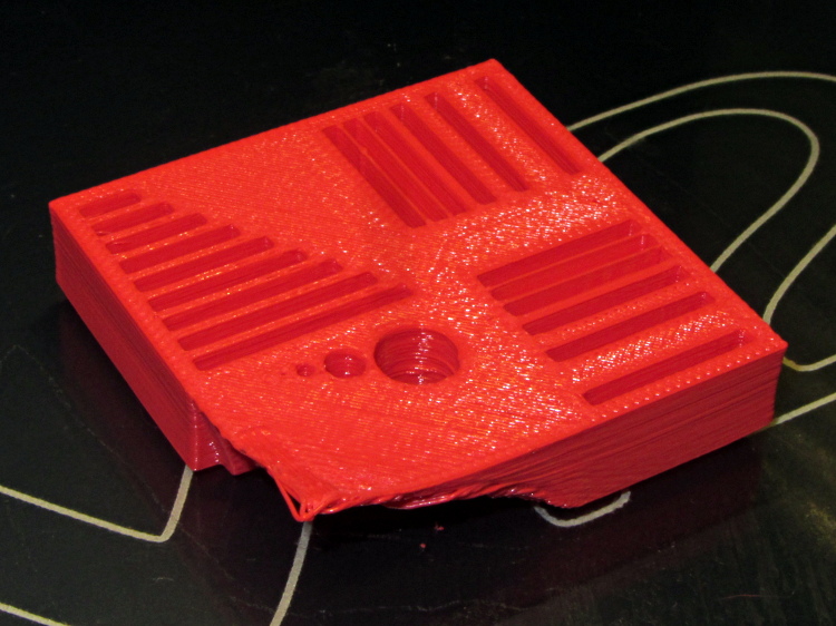
While pulling together a talk on OpenSCAD modeling (more on this later), I ran off a batch of calibration and “torture test” objects, with the intent of seeing how my somewhat modified M2 performs. The short answer is that you (well, I) can’t ask for anything better…
That level of as-printed cleanliness is typical: no stringing, no hair, no misplaced globs, no retraction problems. Basically, the plastic shape on the platform matches the mathematical shape on screen.
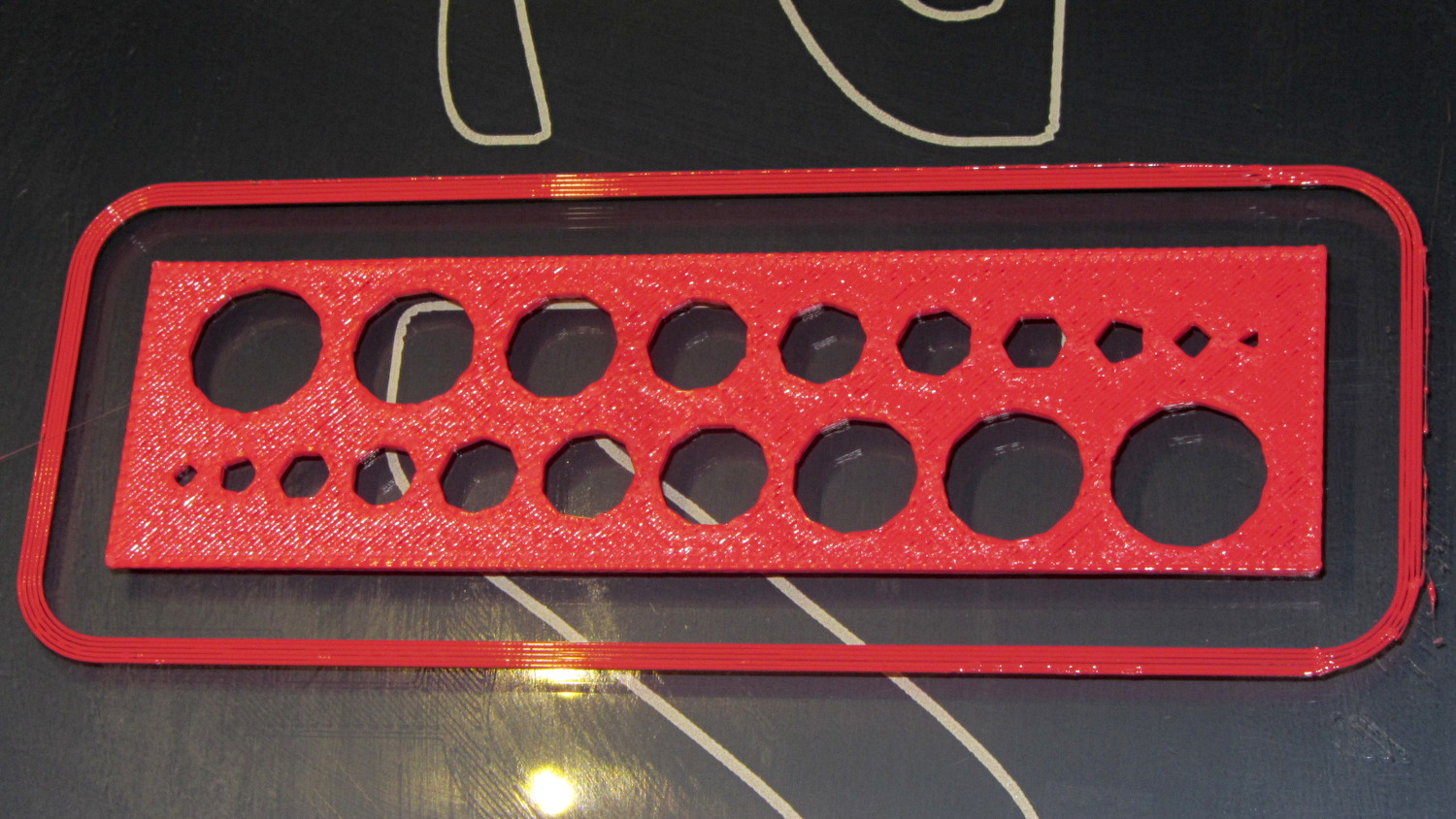
All of the linear features are with ±0.1 mm of nominal; both the 0.5 and 0.25 mm walls came out at 0.40 mm, because that’s the thread width. Slic3r doggedly puts a thread down the middle of hair-fine walls, which I think is a Good Thing.
The holes came out less than 0.3 mm undersize, which is about what you’d expect because they’re not pre-distorted and have far too many sides. The 1.0 and 0.5 mm diameter holes are present, but just barely visible; those simply aren’t reasonable sizes for this technology.
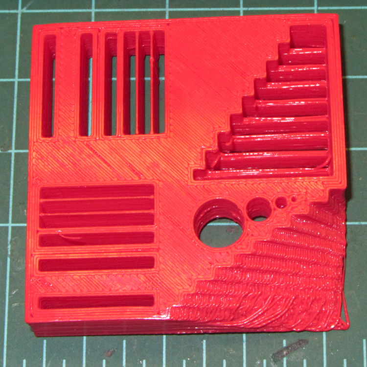
The bottom view shows a few strings in the bridge test area and more detail of the overhang:
M2 – Calibration Block – bottom
Grouping the overhangs like that produced a flat surface that tended to curl upward, so the final slopes don’t match the design. In round numbers, the M2 can handle something like a 60° overhang reasonably well.
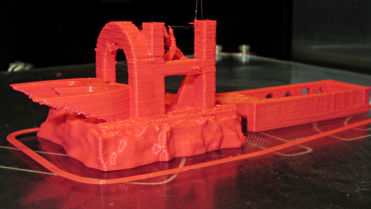
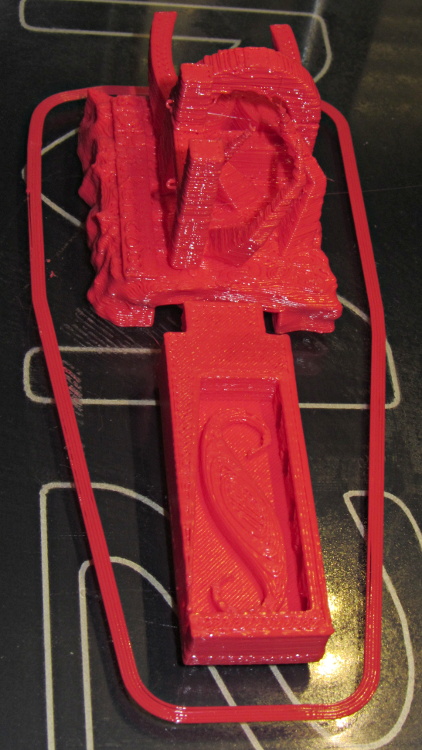
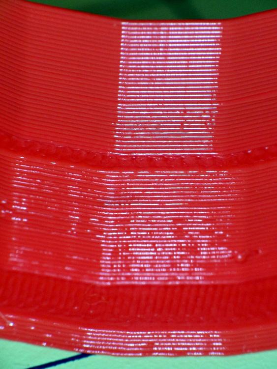
The top view shows the shape in the box looks fine, but with some curls in the main structure. The arch closed over a few random strands, so it’s rougher than I’d like:
M2 – 3DHacker object – top
The spires are lumpy and there’s more striation than I’d like, but this lies well outside the realm of stuff that I build. If I were doing it for real, I’d add some support structures here & there.
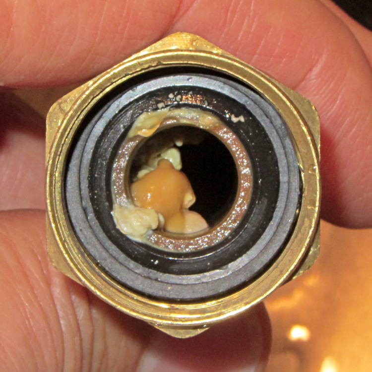
One of my fundamental rules is that you should never, ever look inside the water lines serving your faucets. Having recently replaced a water heater, I had to violate that rule and discovered this growth inside the flex tube at the hot water outlet:
A simple test of additional insulation below the Makergear M2’s heated build platform, measuring the time required to heat the platform from 30 °C to 80 °C:
As-shipped without insulation: 8:20
Cardboard + cotton cloth: 8:30
Cardboard + aluminum foil + cotton: 8:00
That’s with a resolution of about 10 seconds and 1 °C. Ambient temperature was 25 °C; I preheated the platform to 30 °C for a repeatable starting point. The heater was full-on for the entire time and I tried to record the time until it first turned off at the setpoint temperature.
So my initial insulation didn’t make any difference; ten seconds (in the wrong direction!) seems down in the noise.
Adding aluminum improved the situation, but not by much.
The platform wasn’t moving, so there’s no air circulation on either surface. I think it will be possible to record / plot the platform heater duty cycle during printing using LinuxCNC’s HAL components, so some useful data should emerge from that.
I think the bottom line is that there’s so much heat transfer up through the glass plate and away that reducing the heat flow from the bottom by a little bit doesn’t matter…
The original M2 Z axis motor required extremely low acceleration and speed settings, because it produced barely enough torque to lift the weight of the Z stage + HBP + glass platform. The new motor can produce about twice as much torque, so it should perform much better: all of the additional torque can go to accelerating that weight.
I weighed all the bits and pieces while I had the M2 apart, although I forgot to weigh the motor + leadscrew separately:
2.2 kg – Z stage including Z motor
290 g – old Z motor + leadscrew + nut
220 g – motor similar to new motor minus leadscrew
963 g – HBP + glass + clips
So, in round numbers, the whole assembly weighs about 3 kg = 29 N = 6.6 pounds. That’s surprisingly close to my original guesstimate of 3 kg = 7 pounds; I round in the worse direction when there’s only one significant figure.
With the new motor in place, the rods & leadscrew lubed up, and the platform in place, it’s not quite heavy enough to fall under its own weight; it would just barely fall with the old motor. The slightest touch moves it along, though, which means that the angle of friction is just over the lead angle.
The thread form is 30° trapezoidal, so the pitch diameter for an 8 mm OD thread is about PD = 7.2 mm. For an 8 mm lead thread, the lead angle is 19.5° = arctan(8 mm / π · 7.2 mm). Wikipedia’s entry on leadscrews reports the coefficient of friction for oily steel on bronze is between 0.1 and 0.16 for a buttress thread. This thread is trapezoidal, the nut isn’t worn in, the alignment’s probably off a bit, and so forth and so on; so let’s say the angle of friction is 20° and the coefficient of friction is 0.35.
If the new motor can produce, let’s suppose, 500 mN·m of torque, then the upward force on the stage will be:
(2 T) / (PD tan(lead angle + friction angle)) = 1 N·m / (7.2 mm x 0.84) = 165 N
In the ideal world of physics, applying 165 N to a 3 kg stage should accelerate it at 55 m/s2 = 55000 mm/s2 = 5 G.I don’t believe that for a moment, either, particularly because stepper motor torque drops off dramatically at higher speeds.
However, that suggests that, at a rational acceleration, the maximum stepper motor speed could very well be limited by the Marlin 40 kHz step frequency limit to 100 mm/s = (40000 step/s) / (400 step/mm) = 6000 mm/min.
Given that I’m running the XY motors at 5000 mm/s2, I set the Z acceleration to 5000 mm/s2 and discovered that it would stall on the way to 100 mm/s. Backing off to 2000 mm/s2 worked better, so I tweaked the Marlin configuration thusly:
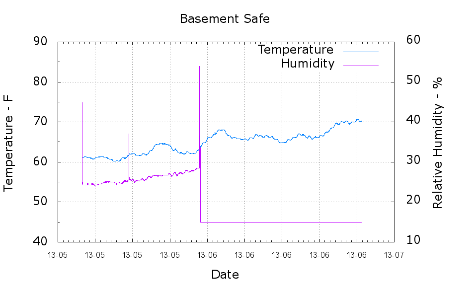
The last two months of temperature and humidity data from inside the basement safe indicate that Spring is becoming Summer down there:
Basement Safe – Temp Humid – 2013-06-30
The new bag of new silica gel beads once again dropped the humidity below the Hobo datalogger’s 15% threshold, so I don’t know the actual humidity. The indicator cards packed inside the silica gel buckets report they’re below 10%; that’s dry enough for me.
However, the bag now weighs 539 g, so it’s pulled 31 g of water out of the air over the last month. The old gel accumulated 63 g over five winter months, so there’s much more water in the air these days! The safe still has a tape seal around the door gap; perhaps a better gasket is in order.
The glitch at the end of May shows the datalogger coming upstairs on a hot, humid day, going back into the safe with the old silica gel tray, then, after a short pause for some Quality Shop Time, snuggling up next to the new bag. The mid-month glitch shows a peek inside the safe…