Ed Nisley's Blog: Shop notes, electronics, firmware, machinery, 3D printing, laser cuttery, and curiosities. Contents: 100% human thinking, 0% AI slop.
Category: Science
If you measure something often enough, it becomes science
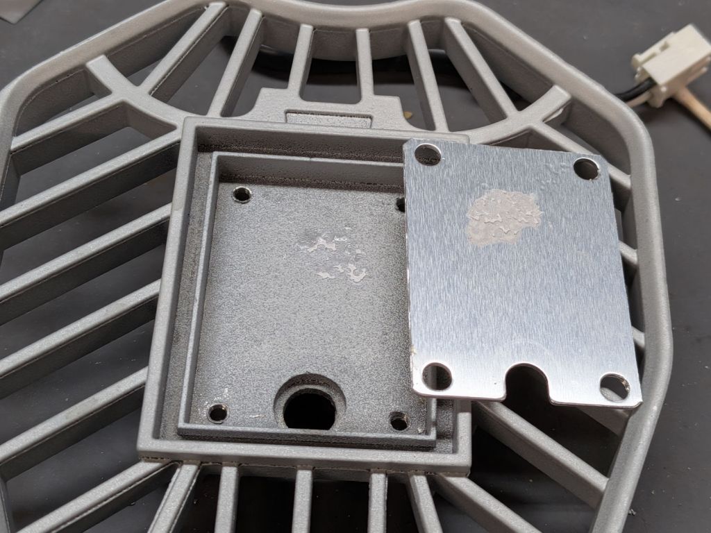
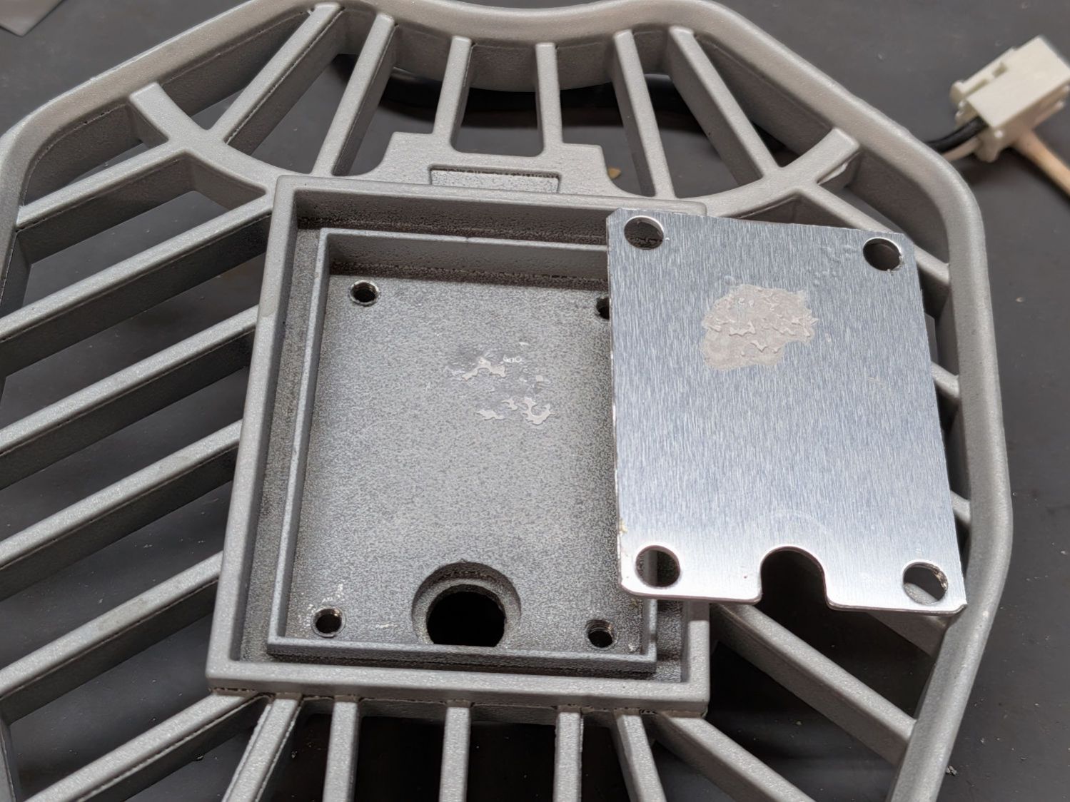
The hidden part of all three LED arrays in the dead garage light looked like this:
LED Garage Light – inadequate heatsink compound
Although the compound was still gooey, there wasn’t nearly enough of it. The few tendrils on the heatsink suggest the LED array had bowed upward, pulled away from the cast aluminum, and eliminated any direct conduction.
A bit of probing showed each LED array had 16 series groups of 4 parallel LEDS, with one group in each array failed open. That group was toward the end away from the inadequate heatsink compound: the LEDs died from heatstroke brought on by neglect.
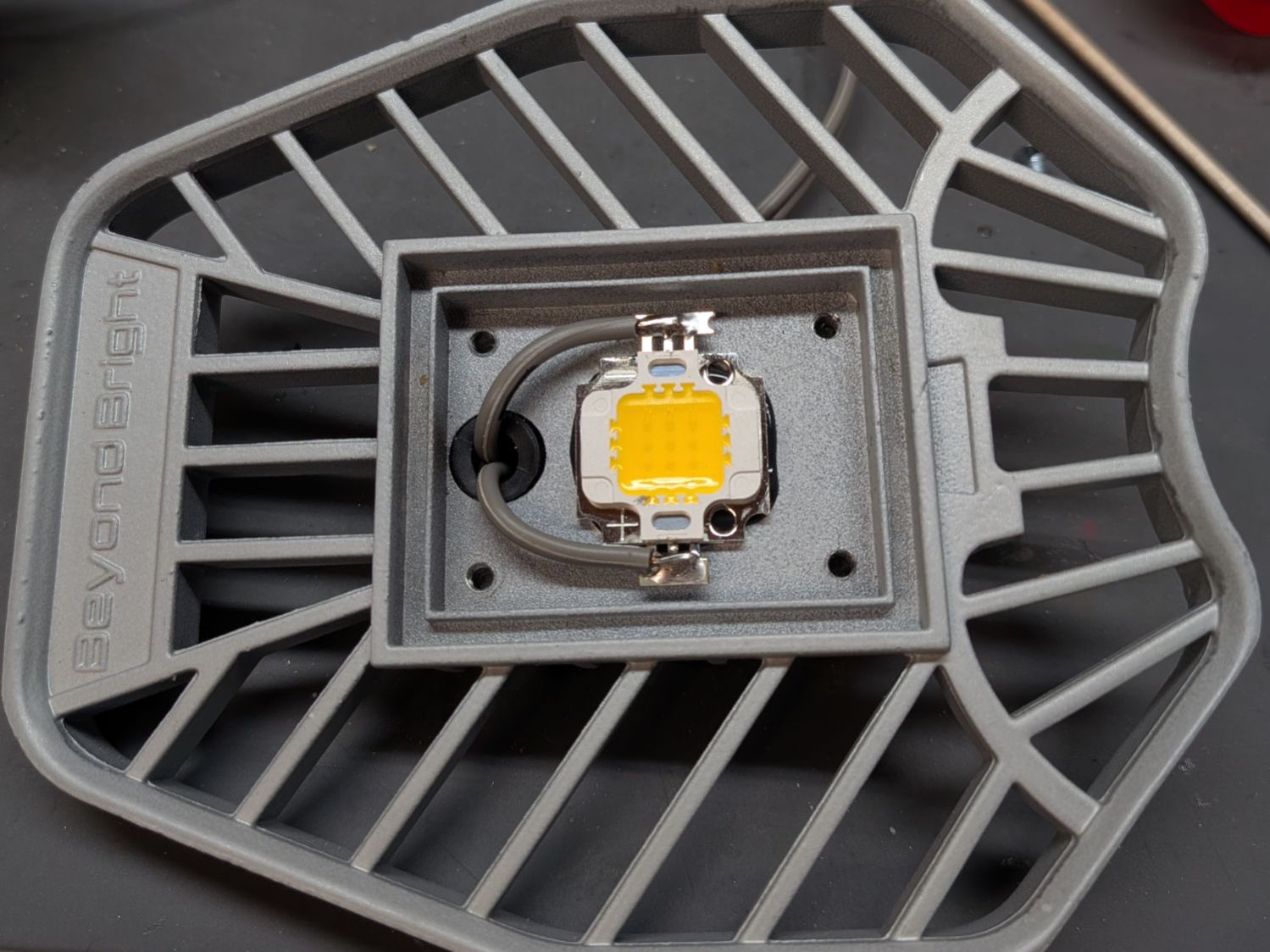
The Drawer o’ LED Arrays disgorged a bag of surplus LEDs labeled “10 W 9-12 V 750 mA”:
LED Garage Light – epoxy replacement
It’s sitting on a generous blob of steel-filled JB Kwik epoxy that should do a great job of conducting heat. A bag of cheap constant-current supplies is on order.
Amazon has similar “10 W 9-12 V 350-450 mA” arrays.
Try as I might, I can’t get 10 W from those numbers, but I’ve never understood advertising math.
The last three boxes had 50 g of activated alumina and got fresh doses from the same bottle.
The other boxes had 50 g from the original bottle of silica gel beads and now have regenerated (and likely damaged) silica gel beads.
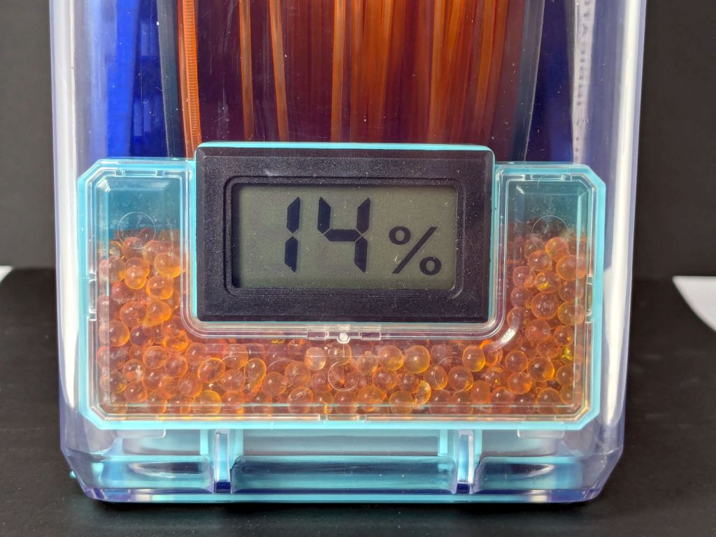
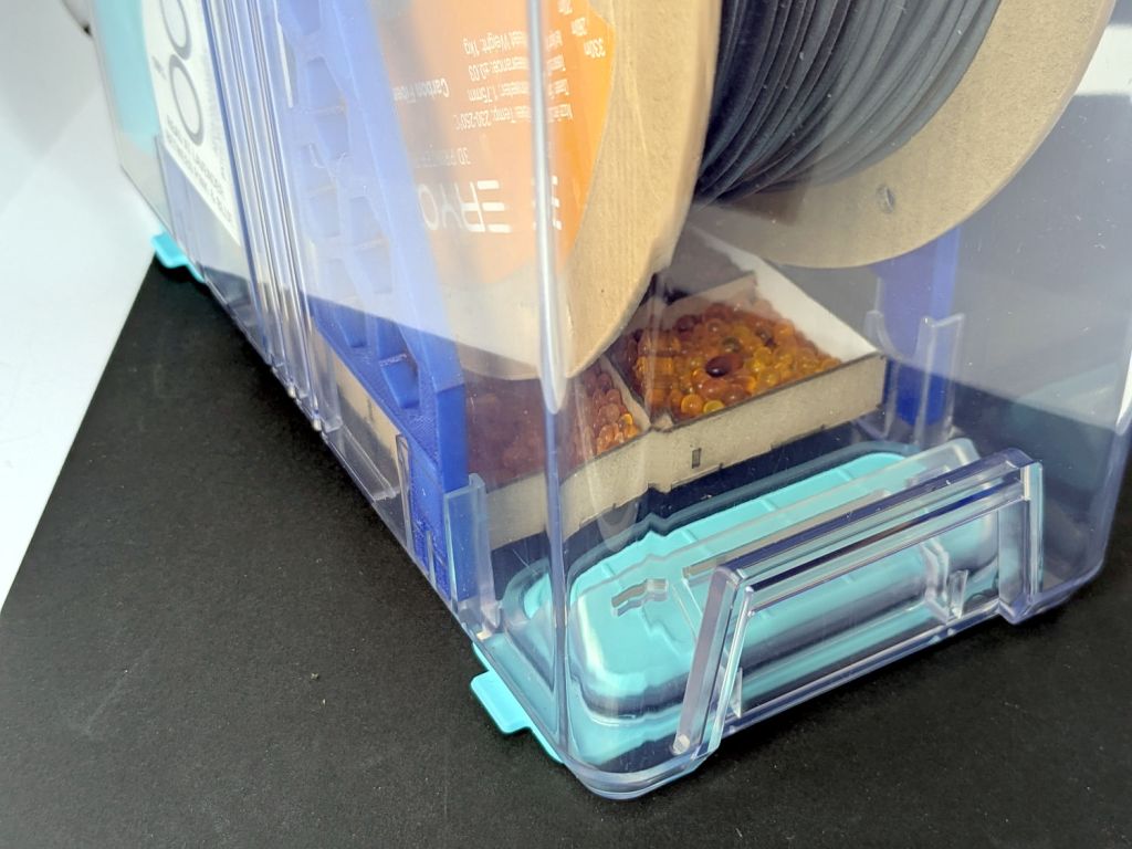
AFAICT, the meter in the orange PETG PolyDryer box isn’t working right, because the humidity indicator card in there has blue spots all the way down to 10%, just like the other boxes. Color differences for meter readings in the teens may be too subtle for my eyes.
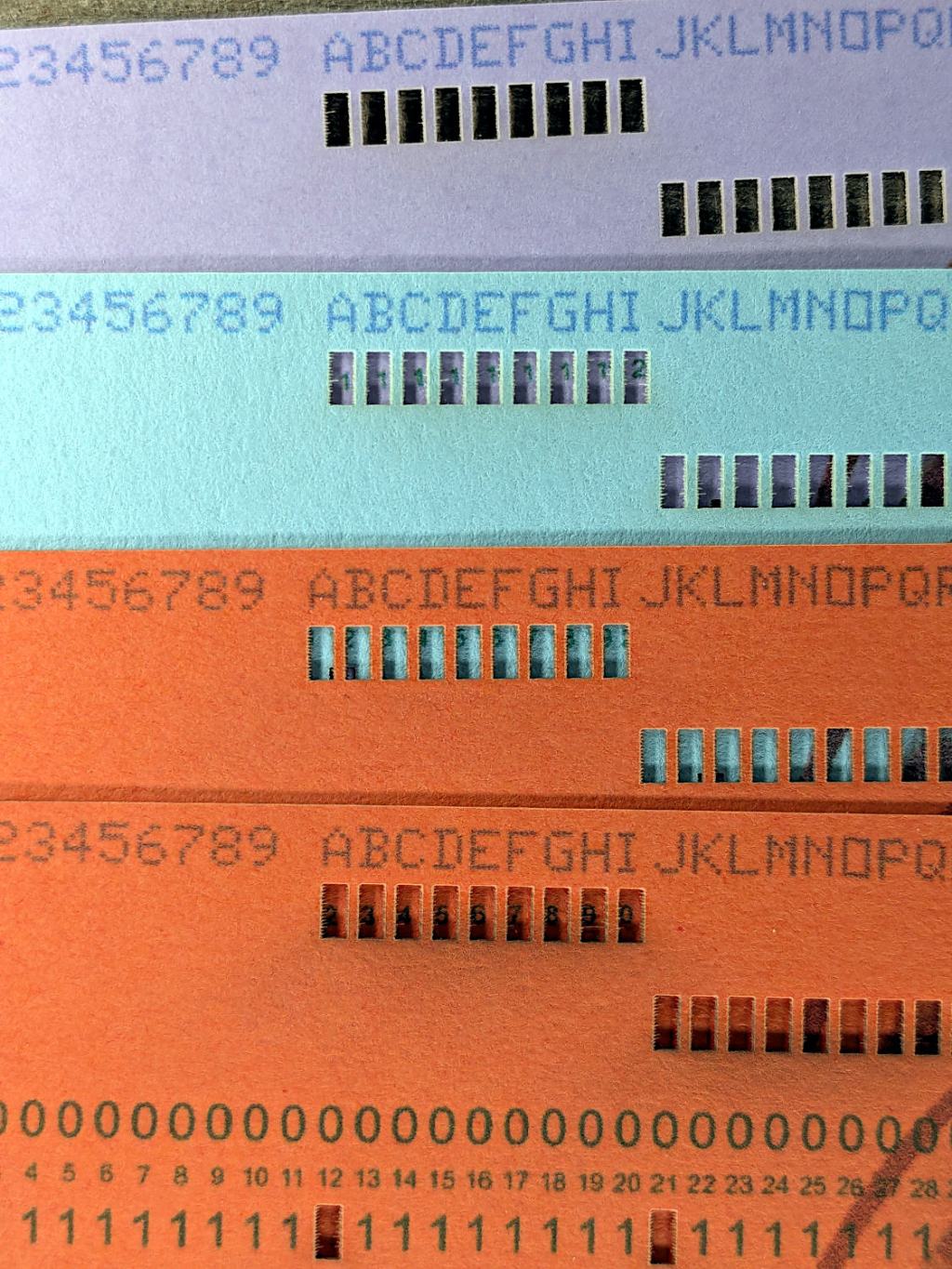
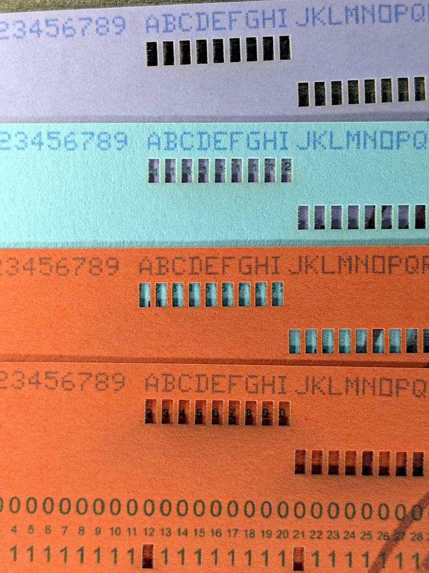
Using different card colors makes it easy to find your program deck in the Comp Center’s output bins:
Punched Cards – paper color vs smoke stains
The smoke stains on the bottom orange card came from the same LightBurn settings used with the purple (violet?) and blue (teal?) cards: 400 mm/s, 35% power, and assist air enabled.
The conventional wisdom is that you *do not* use assist air while engraving, to avoid pushing the smoke / soot down onto the material, and I’ve generally followed that rule. Apparently evaporating holes in the other colors doesn’t generate much smoke and I had no reason to notice the air was enabled.
The upper orange card differs from the lower one only in having the assist air turned off, so I have definitely learned my lesson!
Readers of long memory will recall the dual-path assist air setup that pushes 2 l/m through the nozzle when the LightBurn layer has AIR disabled, specifically to keep smoke out of the nozzle and away from the lens; that gentle breeze doesn’t push smoke into the paper.
FWIW, that’s why I run a set of test cards before I do anything fancy for the first time.
After a few days, it was obvious only the larger beads changed color and, no matter what the description said, they were not going to become any color I would recognize as green.
While the larger ones did get darker, the smaller ones must have already been at their limit of adsorption and remained at the same shade.
For humidity levels under about 20%, I think changing the desiccant every month or so is the only way to be sure.
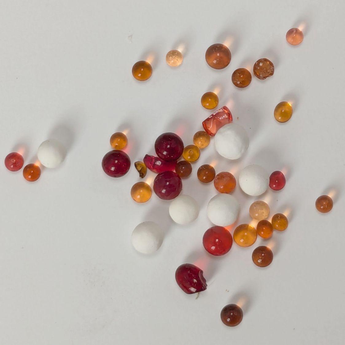
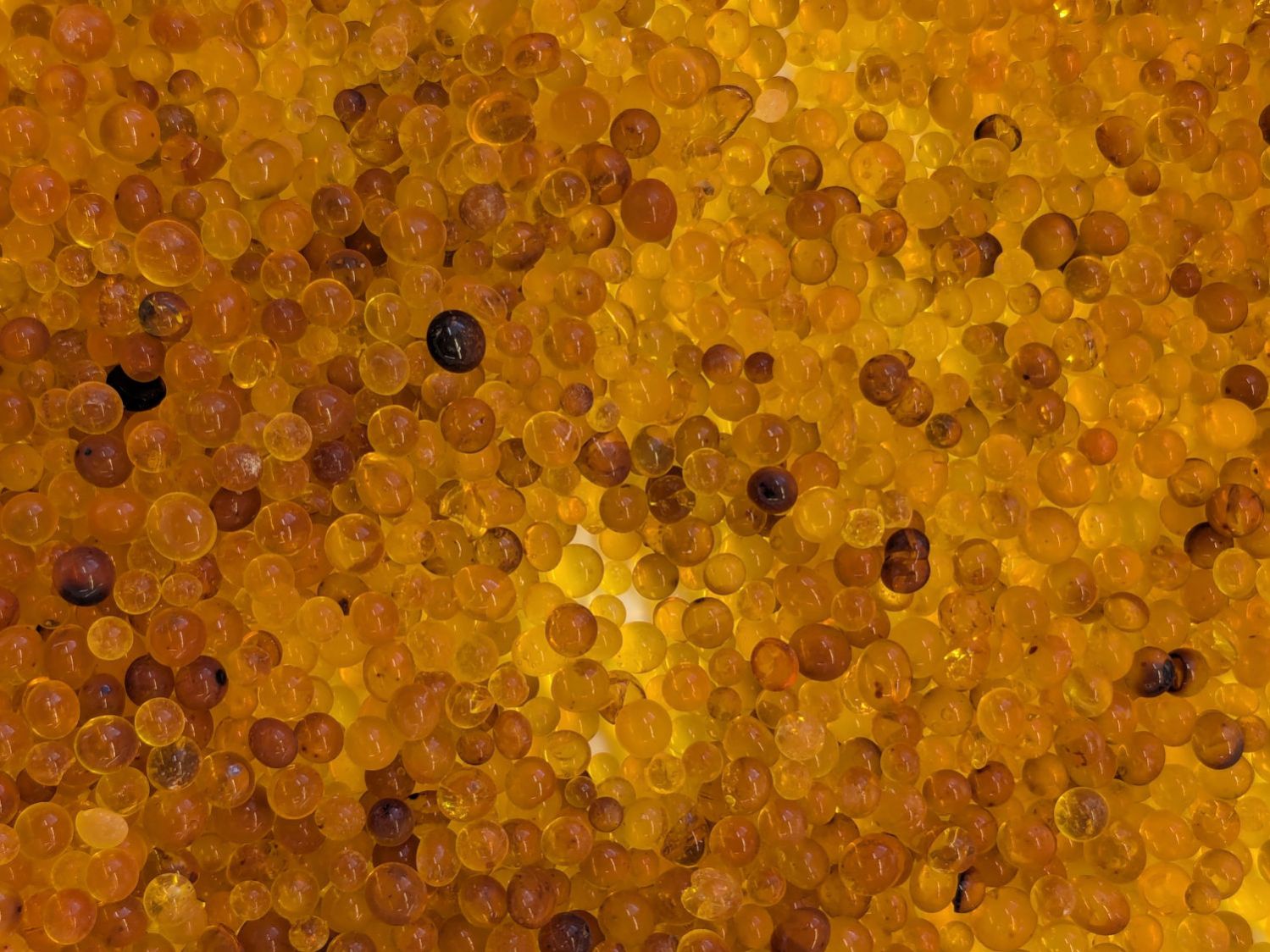
The humidity indicating chemical seems to be methyl violet, described as changing from yellow to green when saturated, which has never happened here. For example, these beads, retrieved from random corners of the workbench, have been sitting in 40-ish %RH basement air for weeks:
Silica gel beads – 36pctRH ambient
The fragment just left of center looks greenish, but the rest are, at best, various shades of brown. This may be due to the (relatively) low humidity in the basement, but putting them under a damp sponge for a few hours didn’t change their color.
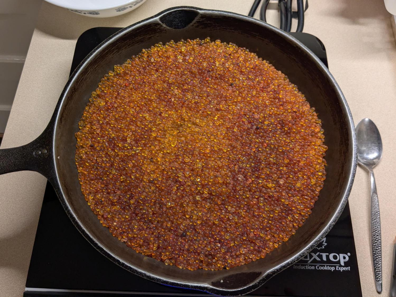
The most recent regeneration session started with an open cast-iron pan on an induction cooktop:
Silica gel beads – drying
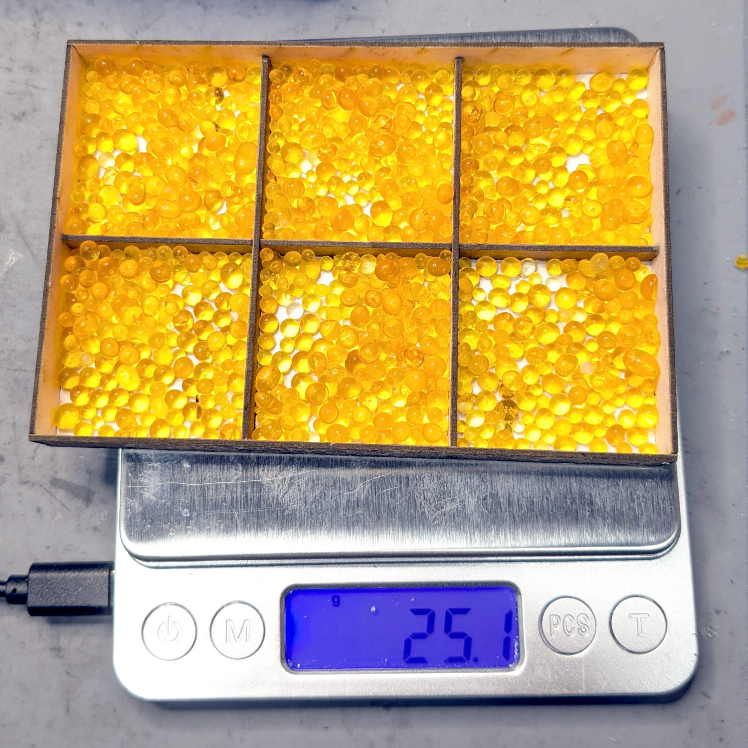
The variety of browns comes from various amounts of adsorbed water in the PolyDryer boxes, but AFAICT there really isn’t much correlation between the humidity level and the amount of adsorbed water.
The drying process went like this:
650 g at start
50% power for 2 hr → 200 °F
Covered the pan & turned it off overnight
623 g at start
50% power for 2 hr → 220 °F
612 g
50% power for 1 hr → 236 °F
610 g
30% power for 30 min → 205 °F
35% power for 30 min → 200 °F
609 g
So about four hours at 50% power would get all but the laser few grams of water out of the silica gel.
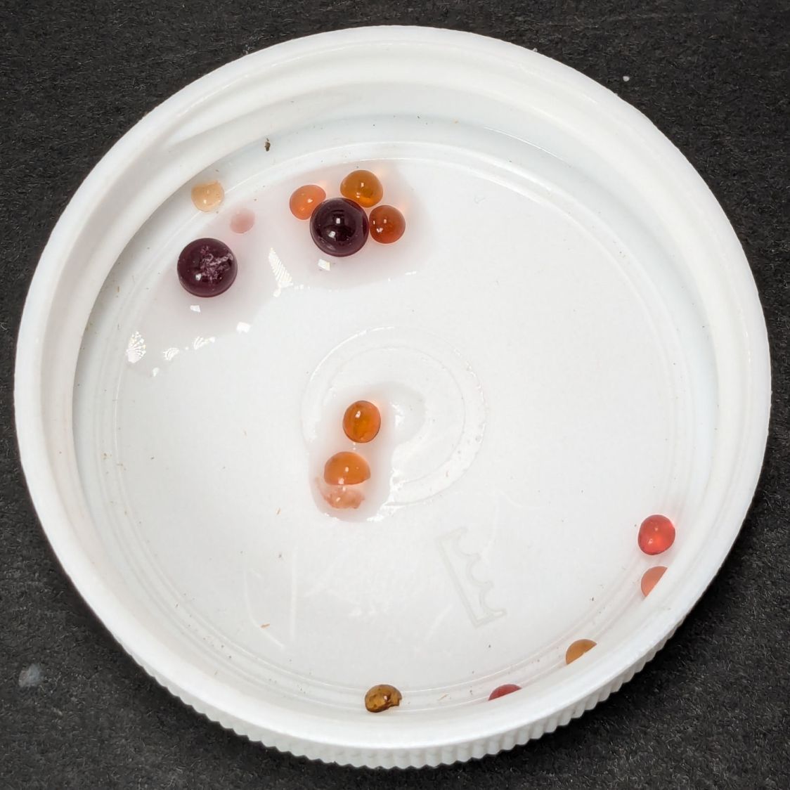
After all that, the beads looked about the same in a white bowl for cooling:
Silica gel beads – damaged indicator dye
Each regeneration cycle leaves more dark brown beads in the mix, which may be due to poor temperature control, and they do not return to their original yellow / pale brown shade.
Apparently cooking silica gel beads over 120 °C = 250 °F (various sources give various temperatures) can damage their structure or the methyl violet indicator; for sure some of those beads have been abused.
Unsurprisingly, the bead temperature rises as they dry out. Although the induction cooktop has a temperature control, we’ve found the setting doesn’t match the pan temperature and the overall control is poor. I could set the gas oven to 200 °F, but I’m certain it doesn’t control the temperature all that closely, either.
The original jug held 2 pounds = 907 g of beads. Add the 609 g from this session to the 350 g of allegedly dry beads in seven of the PolyDryer boxes: my regeneration hand is weak.
I used to think there was some correlation between the indicated humidity and the amount of water adsorbed by the silica gel, with the humidity rising as the gel absorbed more water. That is obviously not the case.
Instead of the adsorption being a function of the equilibrium humidity, it’s the other way around. With the humidity held constant (by adding water vapor), the silica gel will adsorb thus-and-so percentage of its weight and equilibrate at that humidity. If the filament was an infinite reservoir of dampness, then the equilibrium humidity would indicate how much the silica gel had coped with.
At least I think that’s how it goes. I have been wrong before.
Anyhow, IMO the right way to proceed is to just replace the silica gel every month and be done with it.
Also true: the humidity meters aren’t particularly accurate at the low humidity values in those boxes.