Ed Nisley's Blog: Shop notes, electronics, firmware, machinery, 3D printing, laser cuttery, and curiosities. Contents: 100% human thinking, 0% AI slop.
Category: Science
If you measure something often enough, it becomes science
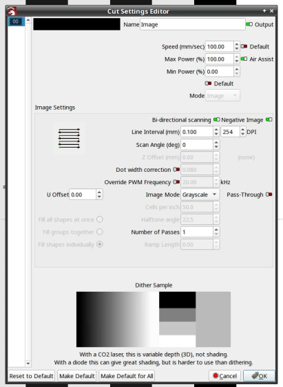
Engrave it in grayscale mode as a negative image with 0.1 mm line spacing:
LightBurn – bandwidth test pattern setup
Monitor the Ruida KT332N controller’s analog laser power control output:
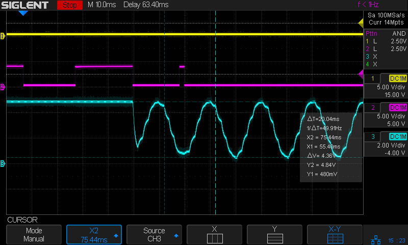
Tube Current – analog bandwidth – 10 sine – 25mm-s – beam off – 254dpi
The traces:
1 X axis DIR, low = left-to-right (yellow)
2 L-ON laser enable, low active (magenta)
3 L-AN analog voltage (cyan)
The scope triggers when the top two traces go low during a left-to-right scan with the laser beam active. The trigger point lies far off-screen to the left, with the delay set to pull the interesting part of the scan into view.
Although both the controller’s L-AN output and the laser’s IN input specify a signal range of 0 V to 5 V, the analog output voltage never goes below 0.4 V, but (as will seen later) that produces 0 mA from the laser power supply.
Set the X cursors to the top and bottom of the sine wave and read off the 4.36 V peak-to-peak value.
Set the Y cursors to matching points on successive cycles and read off ΔT=33.44 ms. Because each cycle is 1 mm wide, the scan speed is set to 25 mm/s and traveling 1 mm should require 40 ms, puzzle over that number and the related fact that 1/ΔT=29.91 Hz. This seems to happen only for speeds under 50-ish mm/s, for which I have no explanation.
Repeat the exercise at various speeds up through 500 mm/s:
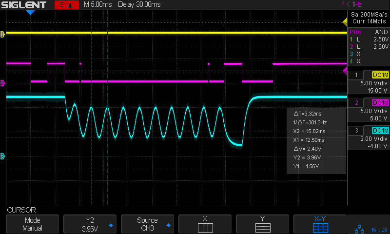
Tube Current – analog bandwidth – 10 sine – 500mm-s – beam off – 254dpi
The analog output voltage has dropped to 1.56 Vpp.
The average voltage increases from 2.66 V at 25 (or is it 33?) Hz to 2.78 at 500 Hz, which is reasonably close to the same value.
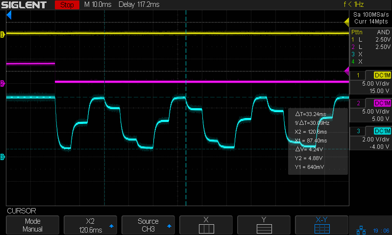
The signal’s -3dB point would be at √½ × 4.36 Vpp = 3.1 Vpp, which happens at 200 mm/s = 200 Hz:
Tube Current – analog bandwidth – 10 sine – 200mm-s – beam off – 254dpi
Then if you tell LightBurn to engrave the pattern with a line-to-line (vertical) spacing of 127 dpi = 5 pixel/mm, it will sample every other pixel in each row, producing a rather peculiar sine-ish wave:
Tube Current – analog bandwidth – 10 sine – 25mm-s – beam off – 127dpi
You must engrave at 254 dpi = 10 pixel/mm in order to get all the pixels in the output stream:
Tube Current – analog bandwidth – 10 sine – 25mm-s – beam off – 254dpi
That still looks gnarly, but it’s more along the lines of what the coarse 10 samples / cycle pattern calls for.
The risetime for each of those steps is on the order of 2 ms, so the controller’s analog output bandwidth isn’t much better than 150-ish Hz.
Close examination of the bar pattern shows the end of the first cycle really does hit exactly 0% intensity where the controller raises L-ON (magenta trace) to force the output current to zero. The other minima remain a few percent above zero and cannot be squashed flat.
Today I Learned: LightBurn enforces square pixels at the line spacing distance for grayscale engraving.
I think this means you must resize / resample the grayscale image to match the engraving line spacing, because LightBurn could take the nearest adjacent pixel or average two adjacent pixels if its horizontal sampling doesn’t match the image resolution.
The pattern gets plunked into the same white/black frame as before, using GIMP because it’s easy.
Importing the resulting PNG image into LightBurn allows configuring the laser parameters. Each sine wave is 1 mm (ten whole pixels!) wide, so engraving at 250 mm/s covers one cycle every 4 ms for a 250 Hz signal:
Tube Current – analog – 10 sine – 250mm-s – 10 ma-div
Changing the engraving speed will change the test signal frequency, although the laser can’t get much beyond 500 mm/s.
The sine wave pattern goes from 0% to 100%, but at 250 Hz the controller output doesn’t reach those extremes, suggesting the output filter rolloff is lower than the 200 Hz inferred from the 1.5 ms risetime and falltime values.
Because the power supply output current isn’t matching the controller voltage excursion and its waveform is much rounder, its bandwidth is even lower.
For example, this would generate five square waves:
Gray bars 10-90
The bars are 10 pixels wide, so scaling the image at 254 dpi makes them 1 mm wide:
LightBurn – bandwidth test pattern setup
As before, the first and last bars are 100% (white), with 0% (black) bars just inboard. The other bars are 10% and 90% to stay a little bit away from the 0 V and 5 V limits. I set Lightburn to invert the colors so that 100% = full power and 0% = beam off.
Engraving the pattern at 100 mm/s makes each bar 10 ms wide and the risetimes and falltimes are easy to see:
Tube Current – analog – gray bars 10-90 – 100mm-s – 10 ma-div
[Edit: Clicked the wrong picture.]
Although it’s a bit handwavy, a 1.5-ish ms risetime suggests a single pole (ordinary RC) time constant τ = 700 µs = 1.5 ms/2.2, so the controller’s output filter cutoff would be around 200 Hz = 1/(2π τ).
The laser tube current looks a little slower than that, so there’s a definite tradeoff among engraving speed, edge crispness, and power level.
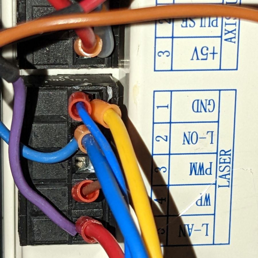
The L-AN terminal produces an equivalent analog signal:
Ruida KT332 – analog laser control wiring
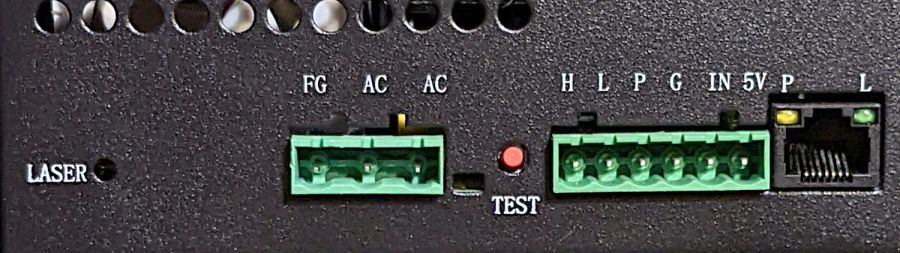
The power supply accepts both analog and PWM signals on its IN terminal, so no rewiring was needed on that end:
OMTech 60W HV power supply – terminals
This test pattern came in handy again:
Gray bars
The pattern has white bars on the left and right edges as markers. I invert the pattern in LightBurn so that white produced 100% PWM and black produced 0% PWM.
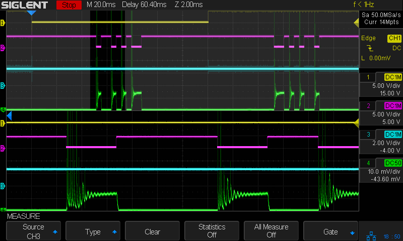
The L-AN output produces 5 V for 100% power and 0 V for 0% power, with other power fractions spread out in between:
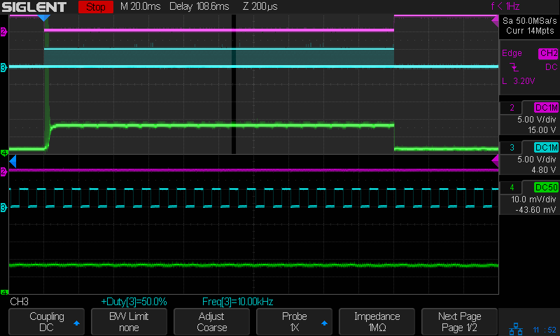
Tube Current – analog – gray bars – 10 ma-div
The traces:
1 X axis DIR, low = left-to-right (yellow)
2 L-ON laser enable, low active (magenta)
3 L-AN analog voltage (cyan)
4 tube current – 10 mA/div (green)
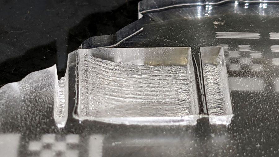
Engraving that pattern in scrap acrylic looks like you’d expect:
Analog mode acrylic engraving
There’s little trace of the discrete intensity levels in the acrylic trench and the scan interval is a rather coarse 0.2 mm.
The PWM signal does not appear in that scope shot, because it runs at 20 kHz and is a blur at 20 ms/div.
It’s worth noting that the tube current has large startup spikes at low power levels in both PWM and analog control, so the spikes are generated internal to the power supply and have nothing to do with the PWM input signal.
Another test pattern using constant power:
Pulse Timing Pattern – 1 mm blocks
At 10% power the analog output is about 0.5 V:
Tube Current – analog – 10pct 250mm-s – 10 ma-div
At 50% power the analog output is a constant 2.5 V and the tube current settles at a constant 12-ish mA, about half of the power supply’s maximum 25 mA:
Tube Current – analog – 50pct 250mm-s – 10 ma-div
Obviously, controlling the laser power to intermediate values using an analog signal does not involve switching the current between the supply’s minimum and maximum values: there are no PWM pulses involved to do the switching.
I suspect the analog output comes from the PWM signal run through an internal low-pass filter similar to the one in the power supply. Based on the PWM frequency measurements and squinting at the rise / fall times, the analog filter cutoff is probably around 1 kHz.
Other than bragging rights, I don’t see much advantage to using the analog signal in place of PWM.
Laser cutter controllers generally set the tube current (and, thus, beam power) through a digital PWM signal to the HV power supply. Confusingly, the same power supply input terminal can receive an analog signal controlling the output current. Both signals have the same 0 to 5 V range.
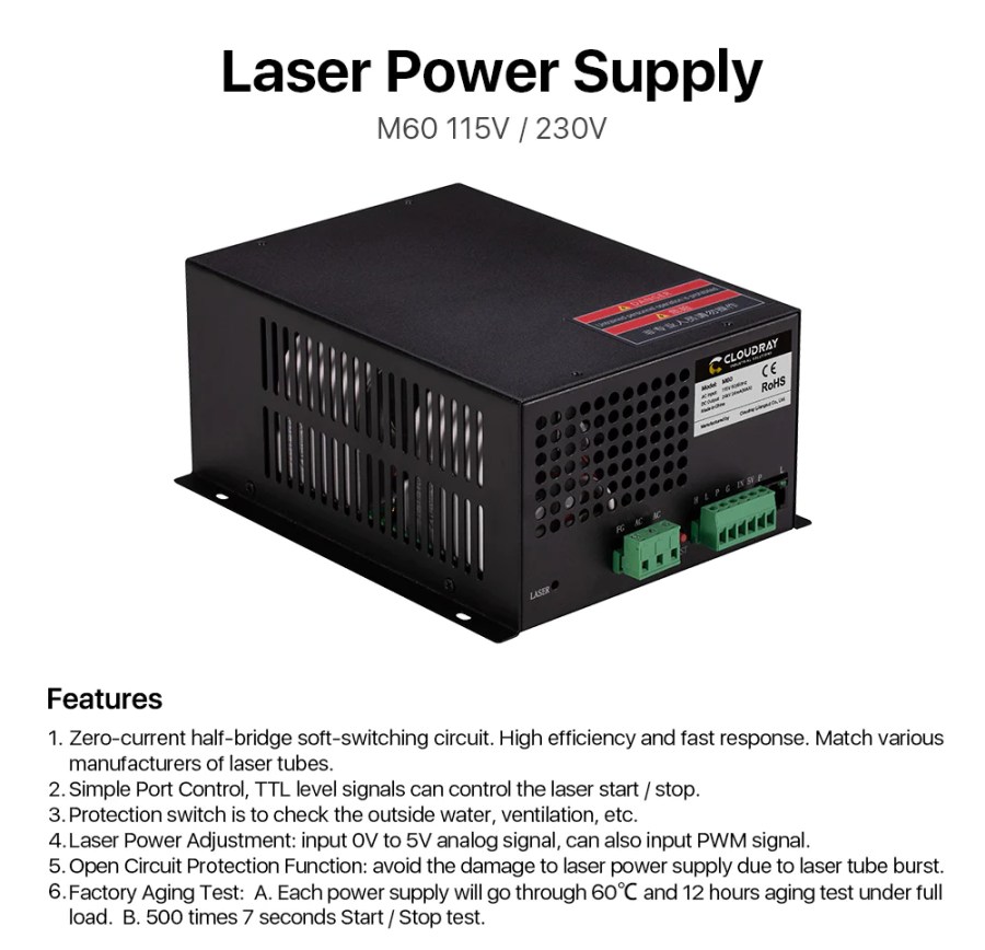
I have yet to see a PWM frequency spec for any HV laser power supply, although surely there must be one. The specs for the Cloudray power supply on my shelf seem typical:
Cloudray Laser Power Supply Features
I have no spec sheet for the replacement power supply OMTech sent, which is now installed in the laser and is measured below. I believe all similar HV laser power supplies, regardless of the nominal brand, are essentially the same inside and will have similar, if not identical, behavior.
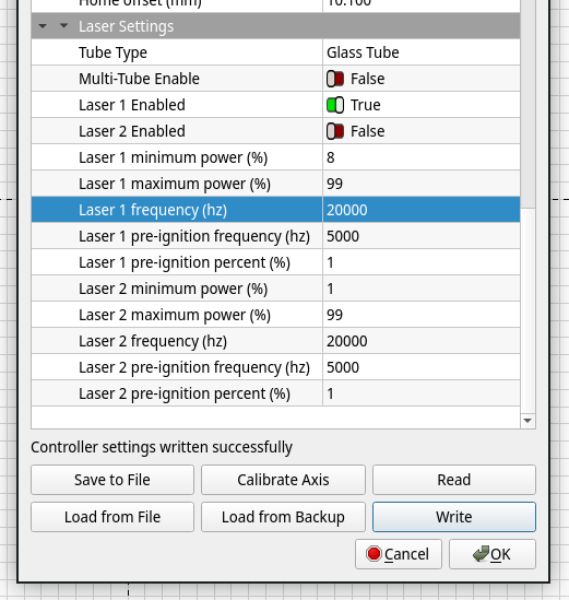
I set the KT332N controller for a 200 ms pulse when poking the front-panel button, which is long enough to show any interesting behavior, and changed the PWM using its awkward controller interface. LightBurn provides access to the “vendor settings” which include the PWM frequency, which I set as needed:
LightBurn Vendor Settings
So, we begin by varying the PWM frequency with a constant 50% PWM …
The default 20 kHz:
Tube Current – 50pct 20kHz PWM – 10 ma-div
The upper half of the scope screen shows the entire 200 ms pulse, with the small slice near the middle appearing zoomed across the bottom half. The readout just above the buttons along the bottom gives the measured PWM percentage and frequency. The green trace shows the tube current is about 12 mA, half of the power supply’s maximum 25-ish mA.
The Tek current amplifier has plenty of thermal drift that I have not attempted to compensate, so always eyeball the average current with respect to the baseline around the pulse in the upper half of the screen.
No trace of the 20 kHz PWM signal appears in the tube current, which runs at a constant 12-ish mA for the duration of the 200 ms pulse.
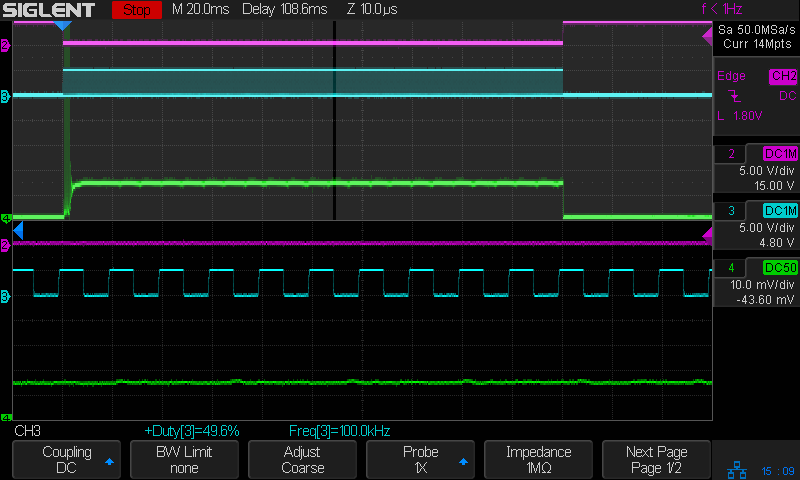
Increasing the PWM frequency to 100 kHz (!) produces no change, although I cranked up the zoom timebase to better show the PWM pulses:
Tube Current – 50pct 100kHz PWM – 10 ma-div
Reducing the PWM frequency to 10 kHz produces very small ripples in the output current corresponding to the PWM cycle:
Tube Current – 50pct 10kHz PWM – 10 ma-div
At 5 kHz the tube current becomes sinusoidal, with an average around the same 12 mA produced at higher frequencies:
Tube Current – 50pct 5kHz PWM – 10 ma-div
The sine wave current is about 90° out of phase with the square wave PWM, although much of that must come from delay through the entire power supply, rather than just an RC low-pass filter.
At 2 kHz the tube current takes on a decidedly lumpy look:
Tube Current – 50pct 2kHz PWM – 10 ma-div
At 1 kHz there’s definitely something odd, perhaps a resonance, going on inside the supply, although the average current remains 12 mA:
Tube Current – 50pct 1kHz PWM – 10 ma-div
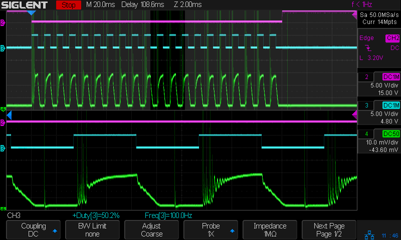
At 500 Hz the PWM is slow enough that the tube current resembles the output of an integrator, rather than a filter:
Tube Current – 50pct 0.5kHz PWM – 10 ma-div
At 100 Hz, the digital PWM signal is so far below the filter cutoff that it’s behaving as an analog input, with the tube current ramping between minimum and maximum:
The current has regular full-on glitches halfway through the “off” part of the PWM signal, so running at absurdly low PWM frequencies does not prevent them. Also note that the PWM signal does not control the current at the same speed as the L-ON enable signal, due to the low-pass filter rolling off the transitions.
Now, holding the PWM frequency constant at (the absurdly low) 100 Hz and varying the % PWM duty cycle …
At 30% PWM, the output current becomes triangular due to the low-pass filter:
At 99% PWM, the output stays at the power supply’s 24 mA maximum output, with small downward ramps marking the 1% off times:
Tube Current – 99pct 0.1kHz PWM – 10 ma-div
Some observations for this HV power supply, which seems typical of similar supplies sporting other “brand names”:
A PWM frequency below 10 kHz introduces output current variations due to the power supply interpreting the PWM waveform as a somewhat analog input, rather than a purely digital signal. This effect increases as the frequency decreases.
An Arduino-speed digital PWM near 1 kHz will be interpreted as an analog signal, with the tube current varying significantly around the PWM signal’s average analog value. It does not control the current in an on-off digital manner.
Due to the effect of the low-pass filter, the PWM signal cannot switch the tube current between “full off” and “full on” at any frequency. The current will always follow a ramp with a slope controlled by the filter rolloff, so low PWM inputs will have low peak currents.
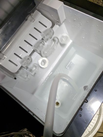
It has a drain hole in the bottom that made this whole thing practical, because a PVC pipe hot-melt-glued atop the drain maintains the water level in the reservoir without any further attention:
Silonn icemaker – drain pipe
The water line from the laser, formerly run directly into the bucket, now goes into the reservoir and through the drain into the bucket. The bucket holds about five gallons of water, with the pump submerged in the bottom.
The icemaker pumps water from the reservoir into the little icemaker tray, freezes nine little ice bullets, and scrapes them into the reservoir:
Silonn icemaker – new ice dump
It does that about every eight minutes.
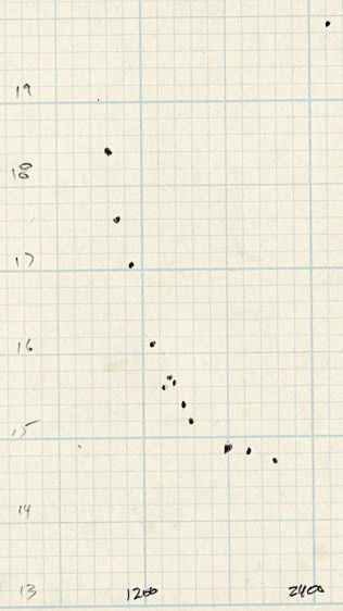
A plot of water temperature vs. time shows what happens:
Silonn icemaker – cooling water plot
It’s as exponential as you could want.
The ice bullets drop into the reservoir and melt there, the cooled water continuously flows into the bucket, and mixes with the rest of the water before being pumped back through the laser. As a result, there are no sudden water temperature changes and the laser remains perfectly happy.
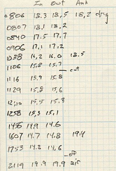
Some numbers for an idea of the cooling capacity:
Freezing 28 pounds = 12.7 kg of ice a day (which, in normal use, would require me to babysit the thing overnight to empty the ice and refill the reservoir) works out to:
12.7 kg × 334 kJ/kg = 4.2 MJ
Spread across 24 hours, that’s 49 W of cooling power. There will be a bit more going into the chilled water surrounding the bullets, but most of the energy goes into the water-to-ice phase change.
Run another way, 5 gallons of water is 42 pounds. The initial cooling slope looks like 2 °C = 3.6 °F in 2 hr, which is 75 BTU/hr = 23 W. However, the water is cooling the laser (which was inert except for one brief cut) as well as the basement, plus (most importantly) there’s a water pump dissipating 20 W submerged in the bucket, so the icemaker is delivering at least 43 W, which is pretty much its rated performance.
It’s obviously incapable of keeping up with a laser doing full-time production work, but for my simple needs it seems better than dunking ice packs in the bucket.
More study (and maybe getting an air-cooled water pump) is in order …