Ed Nisley's Blog: Shop notes, electronics, firmware, machinery, 3D printing, laser cuttery, and curiosities. Contents: 100% human thinking, 0% AI slop.
Category: Science
If you measure something often enough, it becomes science
Well, a shattered lens found beside the road on a walk:
Laser vs sunglasses – focused overview
The battered frame has enough information to suggest they were once rather fancy. At this point, all that matters is they have two glass layers separated by a dark plastic polarizing film, with a gold-ish metallized front glass surface.
I fired the two pulses (on the left side of the obvious crack) at the front of the lens, both at 100 ms / 70% power:
Laser vs sunglasses – overview
Neither pulse penetrated the lens.
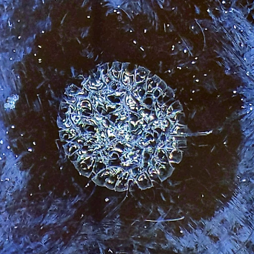
The smaller zit was fired in the position shown in the first picture, with the focal point more-or-less at the top surface of the lens. As seen from the front:
Laser vs sunglasses – focused front
The outer part of the damaged area is about 0.5 mm in diameter. The heat around the damage seems to have cleared away all the schmutz on the lens; those things that look like scratches are oily smears and road dirt.
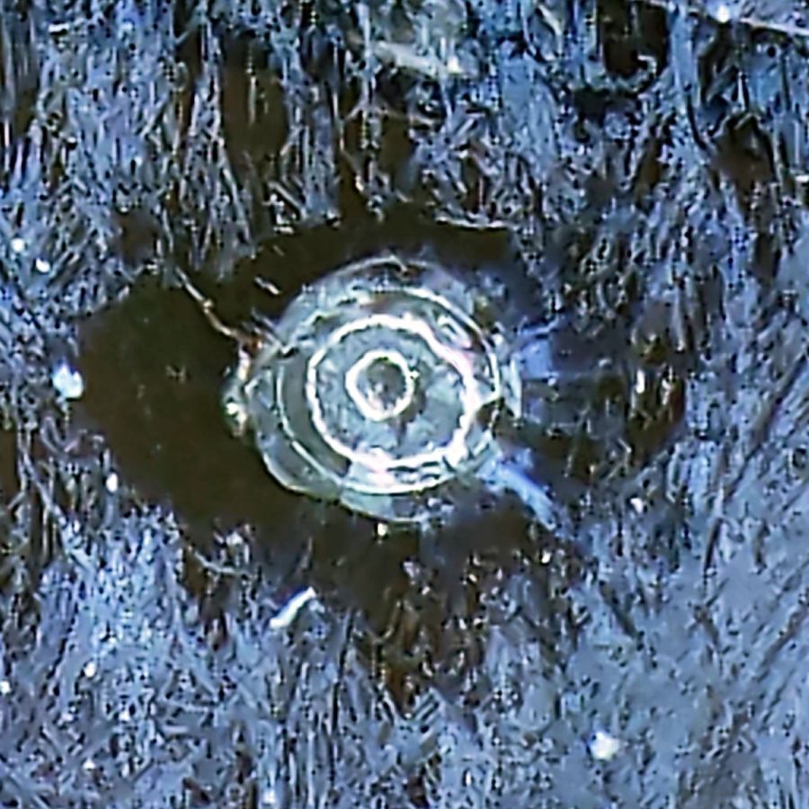
Seen from the rear:
Laser vs sunglasses – focused rear
The rear surface is blistered, but doesn’t have a hole, so I think the beam melted the glass and inflated a cavity along its path.
I then perched the lens in the unfocused beam path, with paper taped over the laser head opening to keep any fragments off the mirror and focus lens:
Laser vs sunglasses – beam front overview
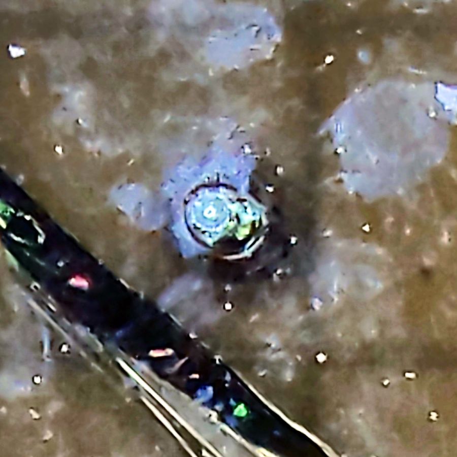
The beam produced the larger scar and also blasted off a ring of crud around the wound, as seen from the front surface:
Laser vs sunglasses – beam front
The beam seems to have shattered a thin layer under the metallization, but didn’t do any deeper damage. The rear surface is undamaged and the paper didn’t have a scorch mark.
They’re not laser safety glasses, but at least they didn’t disintegrate.
Protip: do not lie on the laser platform and stare upward into the laser head, even while wearing fancy polarized mirrorshades.
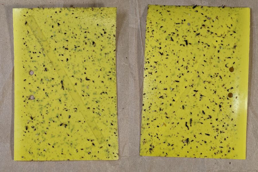
Mary left the sticky card traps in the onion patch until the last onions came out, clustered them around the leeks, and collected them long after the season was over.
I count maybe twenty flies that might be onion maggot flies or cabbage maggot flies.
The cards protected the onion crop, failed miserably for the leeks, and did nothing for the nearby cabbages. Deploying the cards while planting worked very well, refreshing them after a month continued the protection, but the main fly season seems to end shortly thereafter.
All the sticky cards as a slideshow, starting with the three along the border fence:
VCCG Onion Card – fence A – 2022-11
VCCG Onion Card – fence B – 2022-11
VCCG Onion Card – fence C – 2022-11
VCCG Onion Card – plot A – 2022-11
VCCG Onion Card – plot B – 2022-11
VCCG Onion Card – plot C – 2022-11
VCCG Onion Card – plot D – 2022-11
The cards remain sticky to my fingers, but an adroit fly could skate over the debris field and emerge unscathed.
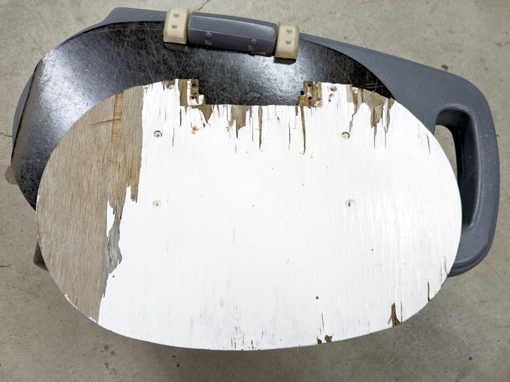
Another tray becomes a replacement for the plywood on the Step2 rolling seat in the Vassar Farms plot:
Step2 Garden Seat – weathered plywood
I reused the old hinges, as this tray seems to be slightly thicker than the one on the home garden seat. The straight edges show it’s also somewhat smaller, but it’ll work just fine.
The bottom of the tray with its Silite logo now faces upward, because the top surface has eroded to a matte finish while supporting a bunch of plants outdoors during several summers:
After two seasons, the first tray doesn’t look any the worse for wear: Silite trays really will survive the Apocalypse and be ready to serve breakfast the next day.
A clipping from the Harrisburg Evening News, probably in 1962, shows more enthusiasm for vaccines than we have today:
Sabin Vaccine Doses – 1962
It emerged from a fat folder of space exploration articles / maps / booklets / clippings with dates from 1959 through 1962, when I would have been around nine years old. Most likely somebody older collected everything and gave the box to me a few years later. The other side had a hagiographic article about John Glenn, explaining why this side is minus a few paragraphs.
From everything I read about Long Covid, I don’t want to give Short Covid even a little bite at my apple. In particular, fast-forwarding through a decade of neural degeneration isn’t going to put me closer to my Happy Place.
The bonus “Volunteer Fireman Convicted of Arson” article could come from any decade.
The usual measurements of voltages and currents assume a constant load impedance, where the power varies with the square of the measured value. In this case, the laser tube is most definitely not a constant resistance, because it operates at an essentially constant voltage around 12 kV after lighting up at maybe twice that voltage. As a result, the power varies linearly with the measured voltages and currents, so the usual Bode plot “20 dB per decade” single-pole filter slope does not apply.
Because the laser tube power varies roughly with the current, I’ve been using the current as a proxy for the power, so the half-power points are where the current is half its value at low frequencies.
The controller’s analog voltage output is linearly related to the tube current and power, so the same reasoning applies.
That reasoning is obviously debatable …
Anyhow, it seems the PWM digital output is the primary signal source, with the L-AN analog output filtered from it. If you had a use for the analog voltage that didn’t involve sending it through a second low-pass filter, it might come in handy, but that’s not the case with the laser’s HV power supply.
Looking across the graph at the tube current’s half-power level of 12-ish mA shows 150 Hz for the L-AN output and 250 Hz for the PWM output. That’s roughly what I had guesstimated from the raw measurements, but it’s nice to see those lines in those spots.
In practical terms, grayscale engraving will operate inside an upper frequency limit around 200 Hz. Engraving a square wave pattern similar to the risetime target requires a bandwidth perhaps three times the base frequency for reasonably crisp edges, which means no faster than 100 Hz = 100 mm/s for a 1 mm bar.
It may be easier to think in terms of the equivalent risetime, with 200 Hz implying a 1.5 ms risetime. The rise and fall times of the laser tube current are not equal and only vaguely related to the usual rules of thumb, but 1.5 ms will get you in the ballpark.
The usual tradeoff between scanning speed and laser power for a given material now also includes a maximum speed limit set by the feature size and edge sharpness. Scanning at 500 mm/s with a 1.5 ms risetime means the minimum sharp-edged feature should be maybe three times that wide: 5 ms / 500 mm/s = 2.5 mm.
The sine bars at 400 mm/s come out very shallow, both rectangular bars have sloped edges, and the 1 mm bar on the left resembles a V:
Sine bars – acrylic – 400 mm-s 100pct
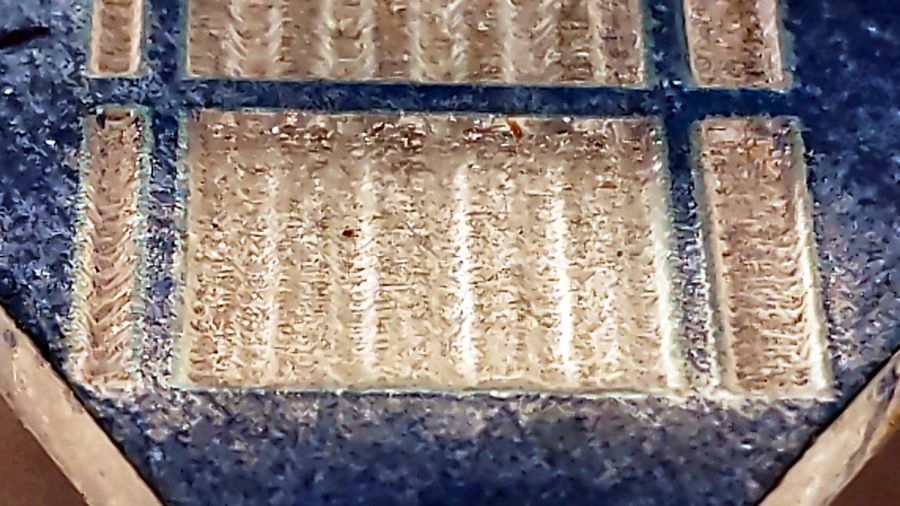
At 100 mm/s, all the features are nicely shaped, although the sidewalls still have some slope:
Sine bars – acrylic – 100 mm-s 25pct
In all fairness, grayscale engraving with a CO₂ laser may not be particularly useful, unless you’re making very shallow and rather grainy 3D relief maps.
Intensity-modulating a “photographic” engraving on, say, white tile depends on the dye / metal / whatever having a linear-ish intensity variation with exposure, which is an unreasonable assumption.
The L-ON digital enable also has a millisecond or two of ramp time, so each discrete dot within a halftoned / dithered image has a minimum width.
Return the laser power supply’s IN terminal (and the purple wire to the oscilloscope) to the Ruida KT332N controller’s PWM output:
Ruida KT332 – PWM laser control wiring
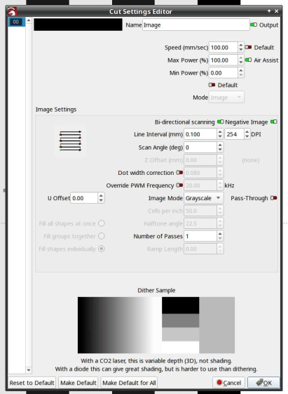
Engraving the pattern in grayscale mode at 254 dpi produces 0.1 mm pixels and makes each bar 1 mm wide:
LightBurn – bandwidth test pattern setup
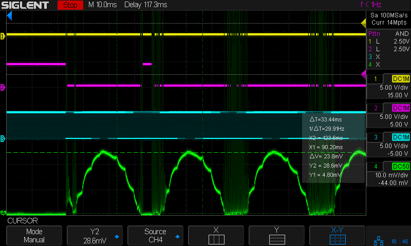
Engraving at 50 mm/s = 50 Hz lets the laser current once again hit full scale:
Tube Current – PWM bandwidth – 10 sine – 50mm-s – 10ma-div – 254dpi
The traces:
1 X axis DIR, low = left-to-right (yellow)
2 L-ON laser enable, low active (magenta)
3 PWM digital signal (cyan)
4 tube current – 10 mA/div (green)
The PWM signal runs at 20 kHz and presents itself as a rather blurred trace, but you can see both the general tendency and the discrete steps between the vertical gray bars. As far as I can tell, the signal never reaches 0% or 100%, most likely to prevent the PWM filters from saturating in either condition.
The tube current drops from 23.8 mA to 13.8 mA, just over the half-power level of 12 mA, at 200 Hz:
Tube Current – PWM bandwidth – 10 sine – 200mm-s – 10ma-div – 254dpi
So the PWM bandwidth is a little over 200 Hz, slightly higher than the analog bandwidth of a little under 200 Hz.
All of the measurements as a slide show:
Tube Current – PWM bandwidth – 10 sine – 25mm-s – 10ma-div – 254dpi
Tube Current – PWM bandwidth – 10 sine – 50mm-s – 10ma-div – 254dpi
Tube Current – PWM bandwidth – 10 sine – 100mm-s – 10ma-div – 254dpi
Tube Current – PWM bandwidth – 10 sine – 200mm-s – 10ma-div – 254dpi
Tube Current – PWM bandwidth – 10 sine – 300mm-s – 10ma-div – 254dpi
Tube Current – PWM bandwidth – 10 sine – 400mm-s – 10ma-div – 254dpi
Tube Current – PWM bandwidth – 10 sine – 500mm-s – 10ma-div – 254dpi
Now, with all the measurements in hand, maybe I can reach some sort of conclusion.
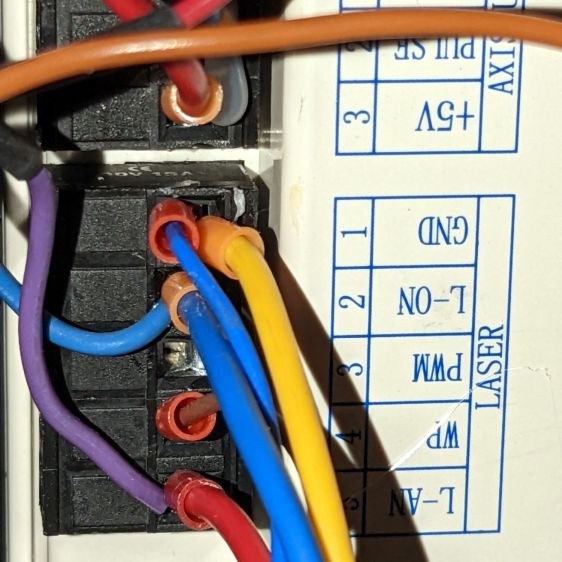
As before, with the Ruida KT332N controller’s L-AN analog output connected to the HV power supply IN terminal:
Ruida KT332 – analog laser control wiring
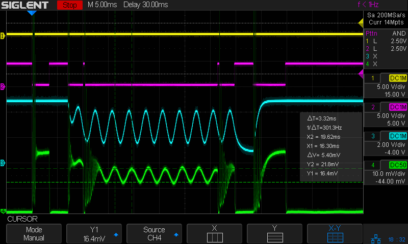
This time the scope traces include both the controller’s output voltage and the laser tube current:
The traces:
1 X axis DIR, low = left-to-right (yellow)
2 L-ON laser enable, low active (magenta)
3 L-AN analog voltage (cyan)
4 tube current – 10 mA/div (green)
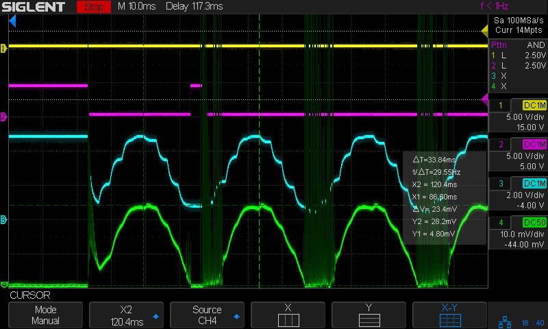
At 50 mm/s = 50 Hz both the L-AN analog voltage and the laser current hit full scale:
Tube Current – analog bandwidth – 10 sine – 50mm-s – 10mA-div – 254dpi
The laser current resembles a damped RLC oscillation when started at nearly full scale and is entirely chaotic when started from zero, but behaves reasonably well for the rest of the cycle.
The power supply’s current bandwidth is definitely smaller than the controller’s voltage bandwidth, as shown by all those sampling steps simply vanishing.
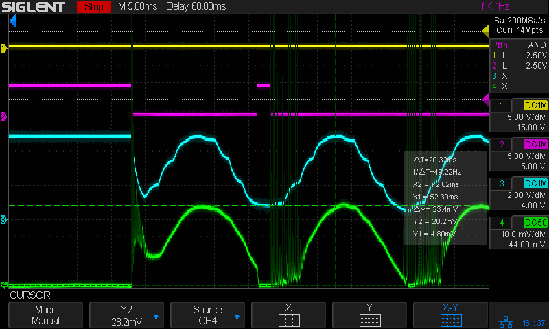
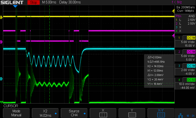
As expected, at 200 mm/s = 200 Hz the L-AN analog voltage is down 3 dB:
Tube Current – analog bandwidth – 10 sine – 200mm-s – 10mA-div – 254dpi
At that frequency the tube current is down 8 dB, from 23.4 mApp to 9.4 mApp, showing how much the power supply’s PWM filter contributes to the rolloff. Since we’re interested in the overall bandwidth, the tube current is down 2.4 dB to 17.8 mA at 100 Hz, suggesting the -3 dB (16.6 mA) frequency is just slightly higher:
Tube Current – analog bandwidth – 10 sine – 100mm-s – 10mA-div – 254dpi
However, I think that’s the wrong way to calculate the -3 dB point of the laser power, because the tube operates at essentially constant voltage, which means both the analog voltage and the tube current are linearly related to the laser tube power, rather than being proportional to its square root.
If that’s the case, then the analog output voltage is down by ½ at 300 Hz and the tube’s half-power point occurs at 23.4 mA/2 = 11+ mA, closer to 200 Hz than 100 Hz. Given the resolution of the measurements, this doesn’t make much difference, but it’s worth keeping in mind.
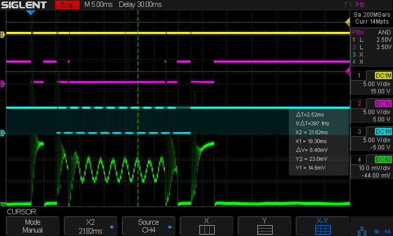
Applying a 100 Hz PWM pulse (thus, a sharp step) to the power supply shows the laser tube current has a risetime (and falltime) around 2 ms, about what you’d expect from a single 200 Hz lowpass filter inside the power supply:
As far as I can tell, the controller’s “analog” output is just its digital PWM output passed through a 200 Hz low-pass filter. It would be useful as an analog input to a power supply without an additional PWM filter, but combining those two filters definitely cuts the overall bandwidth down.
All of the measurements as a slide show:
Tube Current – analog bandwidth – 10 sine – 25mm-s – 10mA-div – 254dpi
Tube Current – analog bandwidth – 10 sine – 50mm-s – 10mA-div – 254dpi
Tube Current – analog bandwidth – 10 sine – 100mm-s – 10mA-div – 254dpi
Tube Current – analog bandwidth – 10 sine – 200mm-s – 10mA-div – 254dpi
Tube Current – analog bandwidth – 10 sine – 300mm-s – 10mA-div – 254dpi
Tube Current – analog bandwidth – 10 sine – 400mm-s – 10mA-div – 254dpi
Tube Current – analog bandwidth – 10 sine – 500mm-s – 10mA-div – 254dpi
To round this out, I must measure the laser tube current bandwidth using the controller’s PWM signal. Because PWM passes through only the power supply’s lowpass filter, the bandwidth should be slightly higher.
Overall, though, the bandwidth seems surprisingly low.