Ed Nisley's Blog: Shop notes, electronics, firmware, machinery, 3D printing, laser cuttery, and curiosities. Contents: 100% human thinking, 0% AI slop.
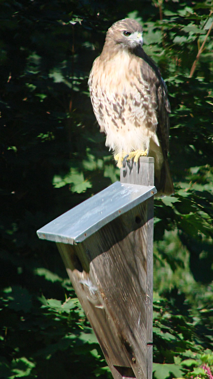
The bird box in the front lawn serves as a favorite perch for surveying the landscape:
Hawk on bird box
The chipmunks seemed fewer and farther between this summer. It’s hard to tell with chipmunks, but they seem to spend more time looking around and less time paused in the middle of the driveway.
Taken with the DSC-H5 and 1.7 teleadapter, diagonally through two layers of cruddy 1955-era window glass.
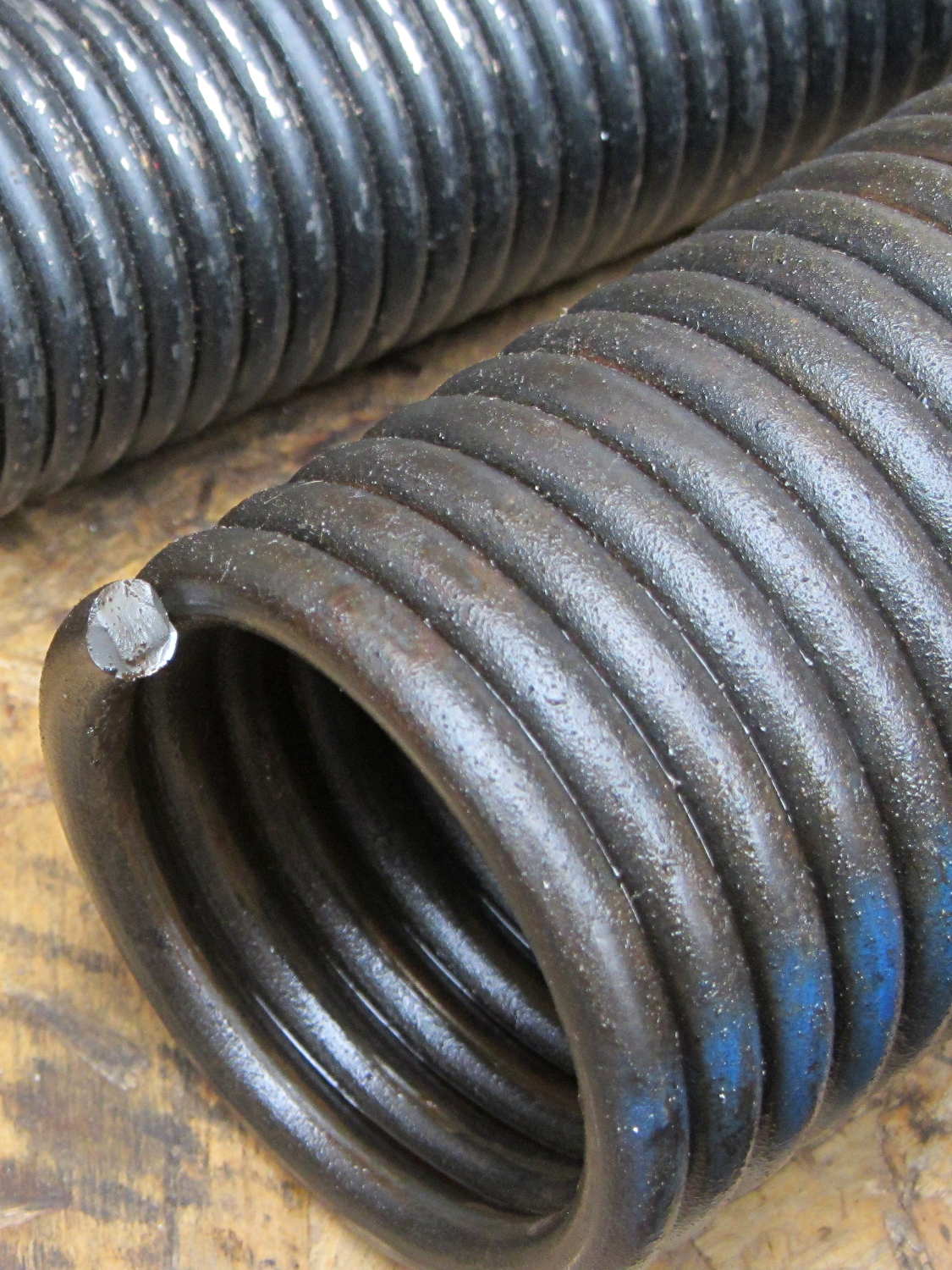
The really good thing about having torsion springs on the garage door is that when one breaks, not much happens:
Garage door torsion spring – broken end
We decided to spray money on the problem and make it go away; the Dutchess Overhead Doors tech was here the morning after I called: quicker than Amazon Prime and he works much faster than I can.
As nearly as I can tell from the checkbook (remember checkbooks?), an original (to us, anyway) spring broke shortly after we moved in. If so, that spring lasted nearly 17 years; at two open-shut cycles per day, let’s call it 12,000 cycles.
For the record, the springs are:
29 inches long
1-3/4 inch ID
0.250 wire
7 foot tall door
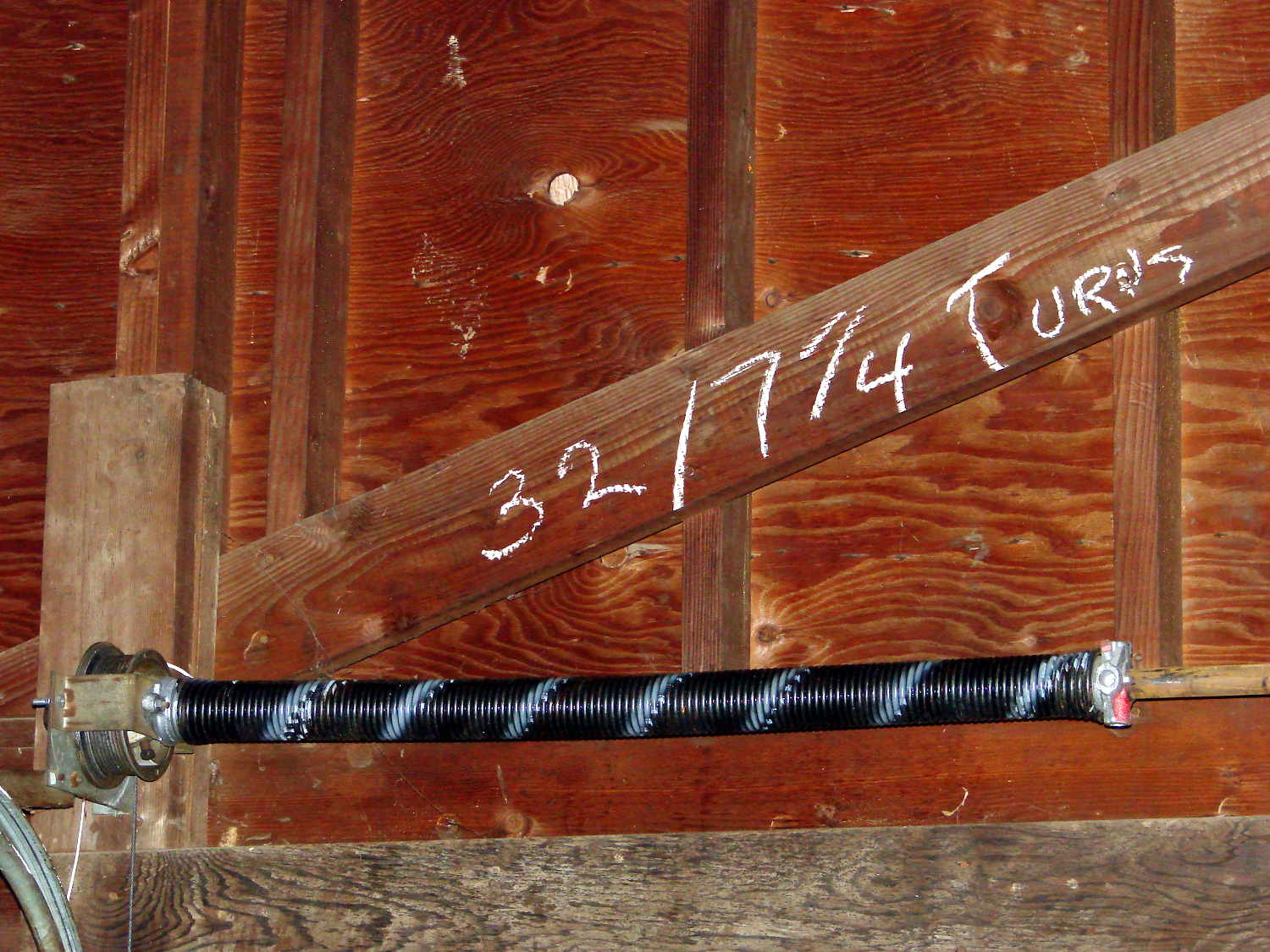
He cranked in seven full turns, corresponding to the “one turn per foot of door height” rule, although the door doesn’t quite balance on its own. I’d have done one more quarter-turn to match the chalk above the door (a good example of write it where you use it), plus maybe another for good measure, but I’m reluctant to mess with success:
Perhaps the 1955 springs were 32 inches long, but the tech replaced what he found both times. It’s a brute of a door, two generous cars wide, with plywood panels in heavy wood framing, plus a few pounds of filler I applied to the rather crazed surface before painting it some years ago.
I’m mildly surprised none of the dimensions changed in the last 60 years: the springs, end caps, pulleys, and hardware directly interchanged.
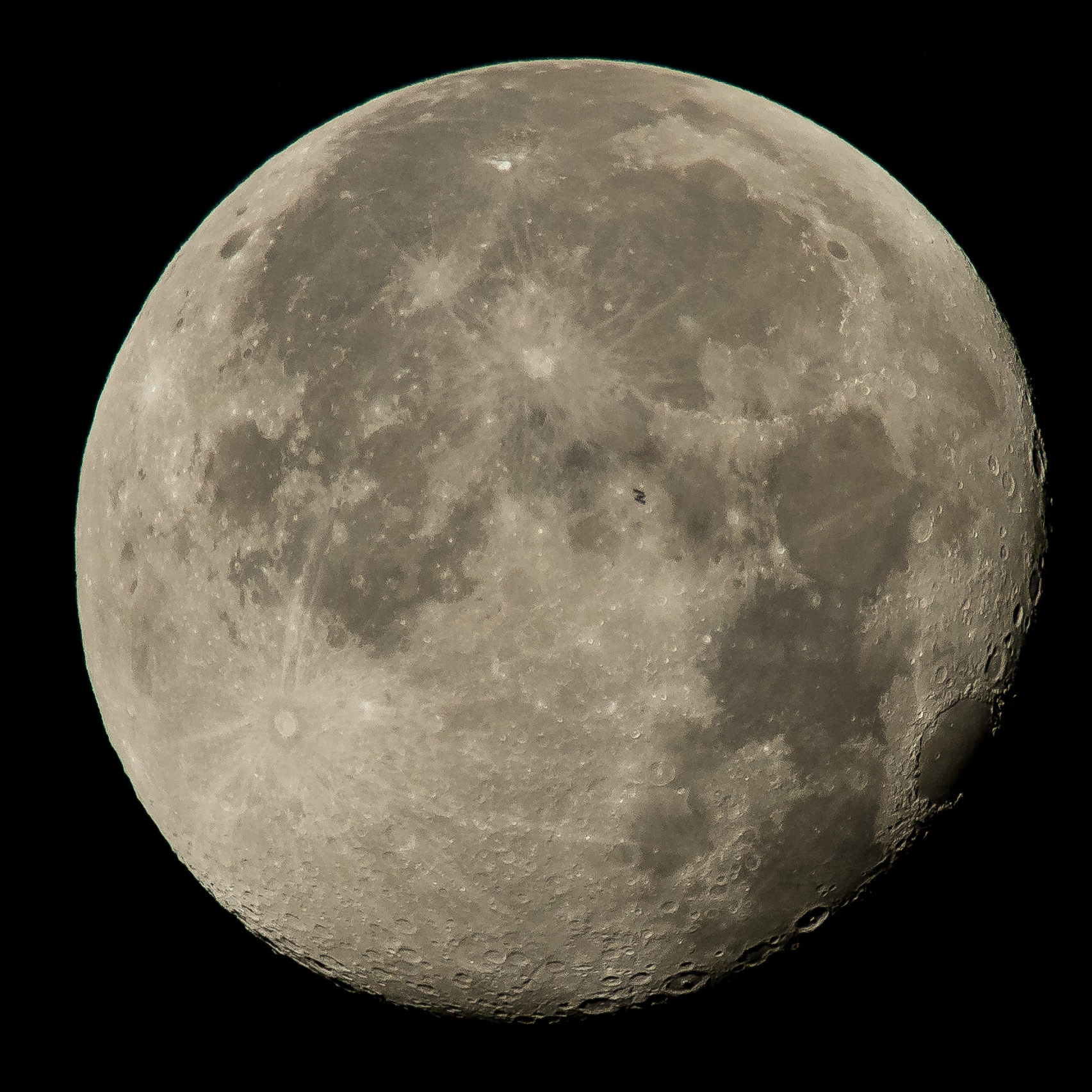
Lunar eclipses happens so rarely it’s worth going outdoors into the dark:
Supermoon eclipse 2015-09-27 2250 – ISO 125 2 s
That’s at the camera’s automatic ISO 125 setting. Forcing the camera to ISO 1000 boosts the grain and brings out the stars to show just how fast the universe rotates around the earth…
One second:
Supermoon eclipse 2015-09-27 2308 – ISO 1000 1 s
Two seconds:
Supermoon eclipse 2015-09-27 2308 – ISO 1000 2 s
Four seconds:
Supermoon eclipse 2015-09-27 2308 – ISO 1000 4 s
Taken with the Sony DSC-H5 and the 1.7 teleadapter atop an ordinary camera tripod, full manual mode, wide open aperture at f/3.5, infinity focus, zoomed to the optical limit, 2 second shutter delay. Worked surprisingly well, all things considered.
Mad props to the folks who worked out orbital mechanics from first principles, based on observations with state-of-the-art hardware consisting of dials and pointers and small glass, in a time when religion claimed the answers and brooked no competition.
ISS Moon Transit – 2015-08-02 – NASA 19599509214_68eb2ae39f_o
The next eclipse tetrad starting in 2032 won’t be visible from North America and, alas, we surely won’t be around for the ones after that. Astronomy introduces you to deep time and deep space.
The relatively low bandwidth of the amplified noise means two successive samples (measured in Arduino time) will be highly correlated. Rather than putz around with variable delays between the samples, I stuffed the noise directly into the Arduino’s MISO pin and collected four bytes of data while displaying a single row:
unsigned long UpdateLEDs(byte i) {

unsigned long NoiseData = 0ul;

	NoiseData |= (unsigned long) SendRecSPI(~LEDs[i].ColB);				// correct for low-active outputs
	NoiseData |= ((unsigned long) SendRecSPI(~LEDs[i].ColG)) << 8;
	NoiseData |= ((unsigned long) SendRecSPI(~LEDs[i].ColR)) << 16;
	NoiseData |= ((unsigned long) SendRecSPI(~LEDs[i].Row))  << 24;

	analogWrite(PIN_DIMMING,LEDS_OFF);			// turn off LED to quench current
	PulsePin(PIN_LATCH);						// make new shift reg contents visible
	analogWrite(PIN_DIMMING,LEDS_ON);

	return NoiseData;
}
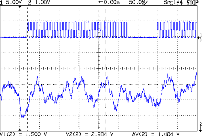
The bit timing looks like this:
SPI Sample – noise data – 01
The vertical cursors mark the LSB position in the first and last bytes of the SPI clock. The horizontal cursors mark the minimum VIH and maximum VIL, so the sampled noise should produce 0 and 1 bits at the vertical cursors. Note that there’s no shift register on the input: MISO just samples the noise signal at each rising clock edge.
I picked those two bit positions because they produce more-or-less equally spaced samples during successive rows; you can obviously tune the second bit position for best picture as you see fit.
Given a pair of sequential samples, a von Neumann extractor whitens the noise and returns at most one random bit:
#define VNMASK_A 0x00000001
#define VNMASK_B 0x01000000

enum sample_t {VN_00,VN_01,VN_10,VN_11};

typedef struct {
	byte BitCount;					// number of bits accumulated so far
	unsigned Bits;					// random bits filled from low order upward
	int Bias;						// tallies 00 and 11 sequences to measure analog offset
   unsigned SampleCount[4];	// number of samples in each bin
} random_t;

random_t RandomData;

... snippage ...

byte ExtractRandomBit(unsigned long RawSample) {

byte RetVal;

	switch (RawSample & (VNMASK_A | VNMASK_B)) {
	case 0:							// 00 - discard
		RetVal = VN_00;
		RandomData.Bias--;
		break;
	case VNMASK_A:					// 10 - true
		RetVal = VN_10;
		RandomData.BitCount++;
		RandomData.Bits = (RandomData.Bits << 1) | 1;
		break;
	case VNMASK_B:					// 01 - false
		RetVal = VN_01;
		RandomData.BitCount++;
		RandomData.Bits  = RandomData.Bits << 1;
		break;
	case (VNMASK_A | VNMASK_B):		// 11 - discard
		RetVal = VN_11;
		RandomData.Bias++;
		break;
	}

	RandomData.Bias = constrain(RandomData.Bias,-9999,9999);
	RandomData.SampleCount[RetVal]++;
	RandomData.SampleCount[RetVal] = constrain(RandomData.SampleCount[RetVal],0,63999);

	return RetVal;
}
The counters at the bottom track some useful statistics.
You could certainly use something more complex, along the lines of a hash function or CRC equation, to whiten the noise, although that would eat more bits every time.
The main loop blips a pin to show when the extractor discards a pair of identical bits, as in this 11 sequence:
SPI Sample – noise flag – 11
That should happen about half the time, which it pretty much does:
SPI Sample – noise flag – 1 refresh
The cursors mark the same voltages and times; note the slower sweep. The middle trace blips at the start of the Row 0 refresh.
On the average, the main loop collects half a random bit during each row refresh and four random bits during each complete array refresh. Eventually, RandomData.Bits will contain nine random bits, whereupon the main loop updates the color of a single LED, which, as before, won’t change 1/8 of the time.
The Arduino trundles around the main loop every 330 µs and refreshes the entire display every 2.6 ms = 375 Hz. Collecting nine random bits requires 9 x 330 µs = 3 ms, so the array changes slightly less often than every refresh. It won’t completely change every 64 x 8/7 x 3 ms = 220 ms, because dupes, but it’s way sparkly.
The noise spectrum at the collector of the NPN transistor looks dead flat:
Noise spectrum – 2N3904 collector
In fact, it’s down 3 dB at 4 MHz, 10 dB at 10 MHz, and has some pizzazz out through 50 MHz.
The cursor marks the second harmonic of the 125 kHz SPI clock that’s shoving bits into the shift registers that drive the LED display. In principle, you can’t get 250 kHz from a 125 kHz square wave, so we’re looking at various & sundry logic glitches that do have some energy there.
The big peak at 0 Hz comes from the LO punching through the IF filters; I should have set the start frequency to 9 kHz (the HP 8591 spectrum analyzer’s lower cutoff frequency) to let the filter get some traction.
With that setup, the first LM324 with a gain of 10 produces this dismal result:
Op Amp 1 10x gain spectrum – 9-209 kHz
Past an op amp’s -3 dB cutoff, the response drops at 10 dB/decade for a while. Squinting at that curve, it’s down 10 dB at 40 kHz and the cutoff looks to be around 4 kHz… not the 100 kHz you’d expect from the GBW/gain number.
[Edit: You’d expect a 6 dB/octave = 20 dB/decade drop from a single-pole rolloff. That’s obviously not what’s happening here.]
The LM324 has a large-signal slew rate of about 0.5 V/µs that pretty well hobbles its ability to follow full-scale random noise components.
Both traces come from a kludged 10 dB AC coupled “attenuator” probe: a 430 Ω resistor in series with a 1 µF Mylar cap, jammed into a clip-lead splitter on the BNC cable to the analyzer. Probably not very flat, but certainly good enough for this purpose.
The SA is averaging 100 (which was excessive) and 10 (more practical) successive traces in those pix, which gives the average of the maximum value for each frequency bin. That reduces the usual hash you get from a full-frontal noise source to something more meaningful.
The LM317 tweaks the reverse bias voltage to ram about 10 µA of DC current through the 2N2907A base-emitter junction; I picked that transistor because it has a 5.0 V breakdown spec that translates into about +8 V in reality, plus I have a few hundred lying around.
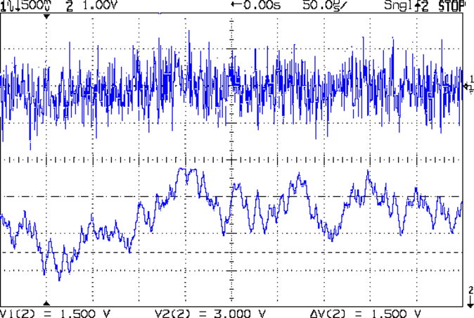
The 4.7 kΩ collector resistor sets the operating point of the 2N3904 NPN transistor at a bit over 6 V with a collector current of 1.6 mA, around which there appears ±500 mV of pure noise:
Noise – NPN C inv – op amp
The 2N3904 spec says hFE > 100 and, indeed, I measure 200: 8 µA in, 1.6 mA out.
The bottom trace is the output of the first LM324. With a GBW of 1 MHz and a voltage gain of 10, it should have a cutoff at 100 kHz, but that’s obviously not true; the 0.5 V/µs large-signal slew rate just kills the response. The flat tops at 3.8 V show that it’s definitely not a rail-to-rail op amp.
The horizontal cursors mark the ATmega 328 minimum VIH and maximum VIL; the actual thresholds lie somewhere between those limits. What you don’t get is the crisp transition from a comparator.
The trimpot setting the logic level lets you tune for best picture; in this case, that means balancing the number of 0 and 1 bits. It’s a bit more complex, of course, about which, more later.
I picked the LM324 for pedagogic reasons; it’s a Circuit Cellar column and I get to explain how a nominally good analog circuit can unexpectedly ruin the results, unless you know what to look for…