CO₂ Laser Tube Current: Analog vs. PWM Bandwidth

With bandwidth measurements in hand, a semilog plot with eyeballometric line fitting makes the conclusion obvious:

The top line shows the controller’s L-AN analog output voltage dropping at 10 dB/decade.

The middle line is the laser tube current with the power supply driven by the controller’s PWM output, also dropping at 10 dB/decade.

The bottom line is the laser tube current with the power supply driven by the L-AN analog voltage. It drops at 20 dB/decade.

The usual measurements of voltages and currents assume a constant load impedance, where the power varies with the square of the measured value. In this case, the laser tube is most definitely not a constant resistance, because it operates at an essentially constant voltage around 12 kV after lighting up at maybe twice that voltage. As a result, the power varies linearly with the measured voltages and currents, so the usual Bode plot “20 dB per decade” single-pole filter slope does not apply.

Because the laser tube power varies roughly with the current, I’ve been using the current as a proxy for the power, so the half-power points are where the current is half its value at low frequencies.

The controller’s analog voltage output is linearly related to the tube current and power, so the same reasoning applies.

That reasoning is obviously debatable …

Anyhow, it seems the PWM digital output is the primary signal source, with the L-AN analog output filtered from it. If you had a use for the analog voltage that didn’t involve sending it through a second low-pass filter, it might come in handy, but that’s not the case with the laser’s HV power supply.

Looking across the graph at the tube current’s half-power level of 12-ish mA shows 150 Hz for the L-AN output and 250 Hz for the PWM output. That’s roughly what I had guesstimated from the raw measurements, but it’s nice to see those lines in those spots.

In practical terms, grayscale engraving will operate inside an upper frequency limit around 200 Hz. Engraving a square wave pattern similar to the risetime target requires a bandwidth perhaps three times the base frequency for reasonably crisp edges, which means no faster than 100 Hz = 100 mm/s for a 1 mm bar.

It may be easier to think in terms of the equivalent risetime, with 200 Hz implying a 1.5 ms risetime. The rise and fall times of the laser tube current are not equal and only vaguely related to the usual rules of thumb, but 1.5 ms will get you in the ballpark.

The usual tradeoff between scanning speed and laser power for a given material now also includes a maximum speed limit set by the feature size and edge sharpness. Scanning at 500 mm/s with a 1.5 ms risetime means the minimum sharp-edged feature should be maybe three times that wide: 5 ms / 500 mm/s = 2.5 mm.

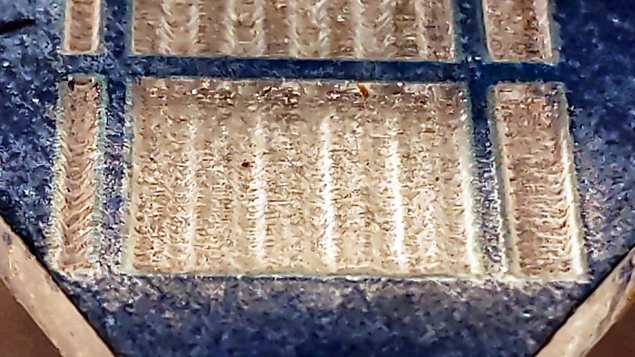
The sine bars at 400 mm/s come out very shallow, both rectangular bars have sloped edges, and the 1 mm bar on the left resembles a V:

At 100 mm/s, all the features are nicely shaped, although the sidewalls still have some slope:

In all fairness, grayscale engraving with a CO₂ laser may not be particularly useful, unless you’re making very shallow and rather grainy 3D relief maps.

Intensity-modulating a “photographic” engraving on, say, white tile depends on the dye / metal / whatever having a linear-ish intensity variation with exposure, which is an unreasonable assumption.

The L-ON digital enable also has a millisecond or two of ramp time, so each discrete dot within a halftoned / dithered image has a minimum width.

Tradeoffs! Tradeoffs everywhere!