The Smell of Molten Projects in the Morning

Ed Nisley's Blog: Shop notes, electronics, firmware, machinery, 3D printing, laser cuttery, and curiosities. Contents: 100% human thinking, 0% AI slop.

Category: Electronics Workbench

Electrical & Electronic gadgets

  • Character-string Histogram

    I’m in the midst of counting glitches on a WWVB receiver, a glitch being any pulse with a duration that isn’t close to 200, 500, or 800 ms. It’s useful to know the pulse width distribution, which is what a histogram does for a living.

    Rather than a graphic histogram, though, I’ve been using a character array (a string!) with one character for each possible pulse duration, measured in units of 20 ms. The value of each character indicates the number of pulses having that duration during the previous minute.

    The counting sequence goes like this:

    • No counts: . (a period)
    • 1 to 9 counts: 1 .. 9
    • 10 to 35 counts: A .. Z
    • 36 to 61 counts: a .. z
    • More than 61 counts: !

    So a minute with no glitches (and a valid WWVB time code frame) looks like this:

    .........4S9............462............322.........
    

    The three clusters show the three valid pulse widths. The pulse widths from the receiver have an inherent jitter, plus the usual ±1 jitter you get for free when you digitize something, plus (this being RF from half a continent away) whatever the Lords of Cosmic Jest do to the signal. So each width usually occupies two or three cells.

    • The 200 ms binary zero pulses form the cluster on the left: that “S” is equivalent to 10 + 18 = 28 counts. Add in the 4 and 9 on either side and you get 41 binary zero pulses.
    • The middle cluster has the 500 ms binary 1 pulses: 4 + 6 + 2 = 12.
    • Each WWVB time code frame has exactly seven 800 ms frame markers, which form the cluster on the right end: 3+2+2 = 7.

    Add them up: 41 + 12 + 7 = 60. That’s exactly the right number of pulses in a minute. What a pleasant surprise!

    A minute with three out-of-spec glitches looks like this:

    1...1....6NC2............82.......1.....51.........
    

    And a minute with very high noise that pretty much obliterates the WWVB signal:

    f!!jHC6AB746312.2121..2.1..........................
    

    Here’s how all that works…

    The histogram counters form a character array that’s also a string. There are 50 20-ms Jiffies in each second (given by the obvious constant), so the histogram has 52 entries: 50 valid counts (0-49), 1 for “more than that”, and 1 for the null byte at the end of the string.

    char    Durations[JIFFIES_PER_SECOND + 2];
    

    Initialize each counter (character) with the starting value and jam a binary zero at the end:

    memset(Durations,'.',sizeof(Durations)-1);
    Durations[sizeof(Durations) - 1] = 0;
    

    And then tick the appropriate counter as each pulse arrives:

    Index = min(PWM_Width,sizeof(Durations)-2);
    
    switch (Durations[Index]) {
     case '.' :
     Durations[Index] = '1';
     break;
     case '9' :
     Durations[Index] = 'A';
     break;
     case 'Z' :
     Durations[Index] = 'a';
     break;
     case 'z' :
     Durations[Index] = '!';
     break;
     case '!' :
     break;
     default :
     Durations[Index]++;
    }
    

    The switch statement maneuvers the counting sequence through the digits, uppercase and lowercase alphabet, then enforces a stall at the maximum count value of “!”. You can’t just increment each element without some checking, because you do not want unprintable control characters in the string.

    Then you print the histogram as you would any ordinary string. If you’re using an Arduino, as I am, this will suffice:

    Serial.println(Durations);
    

    All this depends on the ASCII character set’s numerical sequence. Ponder the charts there and all should become clear.

    Here are the histograms from an hour of WWVB reception during the late afternoon of New Year’s Day: watch the noise floor rise up and eat the WWVB signal…

    
    .........7OD............36............133..........
     .........BID1...........37.............6.1.........
     .1.......9O91..........262.............43..........
     ........27V2............272............421.........
     .........4Y41...........46............124.........2
     .........AP71...........2811..........123.........2
     .........AN9............731...........1.6..........
     12.111..28IB11.........1623.......2..1.42.....2....
     1412...125Q911..........461.....1......41..........
     1........8Q81..........137...1.........15..........
     .12....119N912.........116..........1.132..........
     1521..1.17O931...1......27...........1..5..........
     .12....12BKB2...........332....1......132.......2..
     25211.1.3AHB5......1...1143........1...14.........3
     45412...4BDA4..12.......25111..1.....1..22.........
     6A44322.26CI53.2.1...1..343...1.......1.11.........
     5D75531113FG511...12..212313.1........1.2..1.......
     1432.1.119GB41..........262.1...11.....14..........
     .5211..115MB4...........441............14.2........
     .4.1....25JB6...........442.........1..231.........
     6B443...27I772..........2322.....1.....1221......2.
     4555411.27HA321........3232......1....114..........
     3232.1.129GI1...1.......4321...1.1.1...111.........
     ...1..1.19O8..1....11...262............24..........
     11......2AN62...........622...........124..........
     111.....2BJ551..1......1522........3..141........21
     1421....29N611.......1.136............1231........2
     1.12.....AIB3........1..38...1........312..........
     7F42..1.28FE341.1.1.....351........1...12...1.....2
     .23......8GG2....11....2423............33..........
     112..13.1AK931.....2....142....2.11.1..3.1........2
     423111..44JD4.2..1.....1433........11111...........
     1413..1.3CL812..11......242..1....11...21.........2
     474112.34AI84.2...3.1...16.2.....1...1.11..........
     8LHC734657D857411..11...131......1..1.1...........2
     JuSFDCCDDCD662412...1..............................
     VmG376788AC8671.21.1..3.......1....................
     IlCB4576CFE532131.11.1..1.1........................
     KxN798EB98A7422...2.1...1..........................
     AYL96853CF7742121311.13..21....1...................
     8TDEB6649A7952..32.41..124.....1.....1............2
     DeO78638C9GA6142.15111..........1........2.....2...
     AcPC83426BD4823.122..11132.1.......................
     7SF31121AHFB73..2.111...321..1.1...................
     7F3221414GG5411.111121.133...1.1.1.................
     6RD9669647F7361.31.2..1212...1.....................
     6L71.2444ALB21...221.212321..2...1...1.............
     4LHFD7638C9B12.31341.22113...2..........1..........
     264321112EFA5.112.22.2.14111..1.....1...1.........2
     235511445BEC3.12..1131.131..1.1........11..........
     7UC741635AAC442.1..112.1..11311.......1.1.........2
     EVLCAB3598E752252133.111.1.1..........1...........2
     JnTE9913A59A452331.13..1222.............1..........
     f!!jHC6AB746312.2121..2.1..........................
     !!!iMB772.4532..1.1.1.1..1.........................
    
  • Arduino Serial Optical Isolator

    Optical Isolator - oops
    Optical Isolator – oops

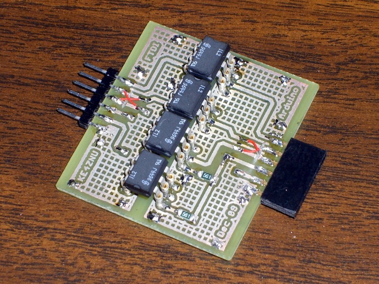
    It turns out that attaching some, but not all, of the PCs around here to the Arduino Pro board controlling the Totally Featureless Clock cause the WWVB receiver to drown in a sea of noise. In fact, just touching the USB cable’s shield to the FTDI Basic USB-to-serial adapter would bring the noise.

    So this is a quick-and-dirty circuit to see if optical isolation will reduce the problem enough to be bearable.

    The schematic is pretty simple: two bits in, two bits out.

    Optical Isolate Schematic
    Optical Isolate Schematic

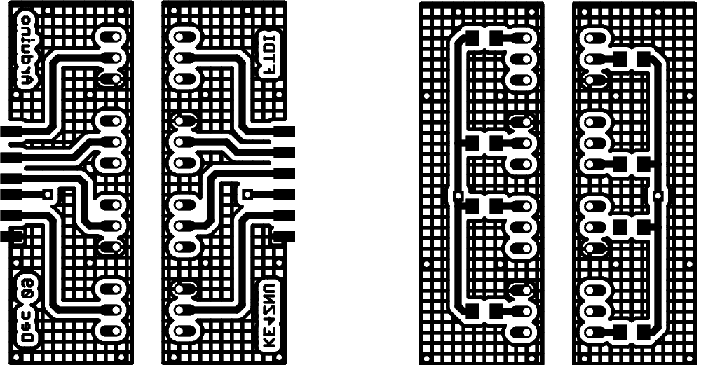
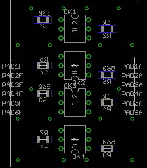
    The layout puts the DIP isolators on the top and the SMD resistors on the bottom. I used fancy screw-machine IC socket pins, just because I had some, but you could solder the isolators directly to the board. The FTDI Basic connects through header pins and the Arduino connects through female header sockets, both soldered sideways to the top of the board. I’ll eventually reinforce them with some epoxy, never fear.

    Double-size PCB layout:

    PCB Layout
    PCB Layout

    Actual-size copper images. Remember that the top copper is flipped left-to-right here so it comes out properly after toner-transfer imaging.

    Copper
    Copper

    And the placement info showing where the parts wind up. This is sort of the silkscreen for the top and bottom, both together: the backwards stuff goes on the bottom side.

    Top and Bottom Silkscreen
    Top and Bottom Silkscreen

    The alert reader will note that the photo doesn’t match the rest of the images. Nay, verily, eagle-eyed readers will have picked out a few resistors on the top and two embarrassing little red-wire Xes at the connectors. Somehow, I managed to swap the RxD and TxD pins, even with an FTDI board on the desk next to me. I hate it when that happens… so I fixed the schematic & layout for the next time around.

    The resistors push a lot of current through the LEDs and phototransistors, which is what you need to get decent 19200 b/s serial data pulses. Here’s what the data stream out of the TxD isolator looks like:

    Optoisolator - TXD
    Optoisolator – TXD

    I have the Eagle files and the CNC drill file for my Sherline mill if you must have them, but you can go from those images above directly to the hardware. It’s an evening’s work, more or less.

    You might want to kludge a jumper into the Reset line so it’s impossible to accidentally reset the Arduino. Sometimes you don’t want a reset, like after a few days of data collection…

    Now, does it actually do what I expected? The early reports are good, but I’m at the mercy of the atmosphere and must collect a few days (actually, nights) worth of data to find just how far down the noise went.

  • WWVB Time Code Format Diagram

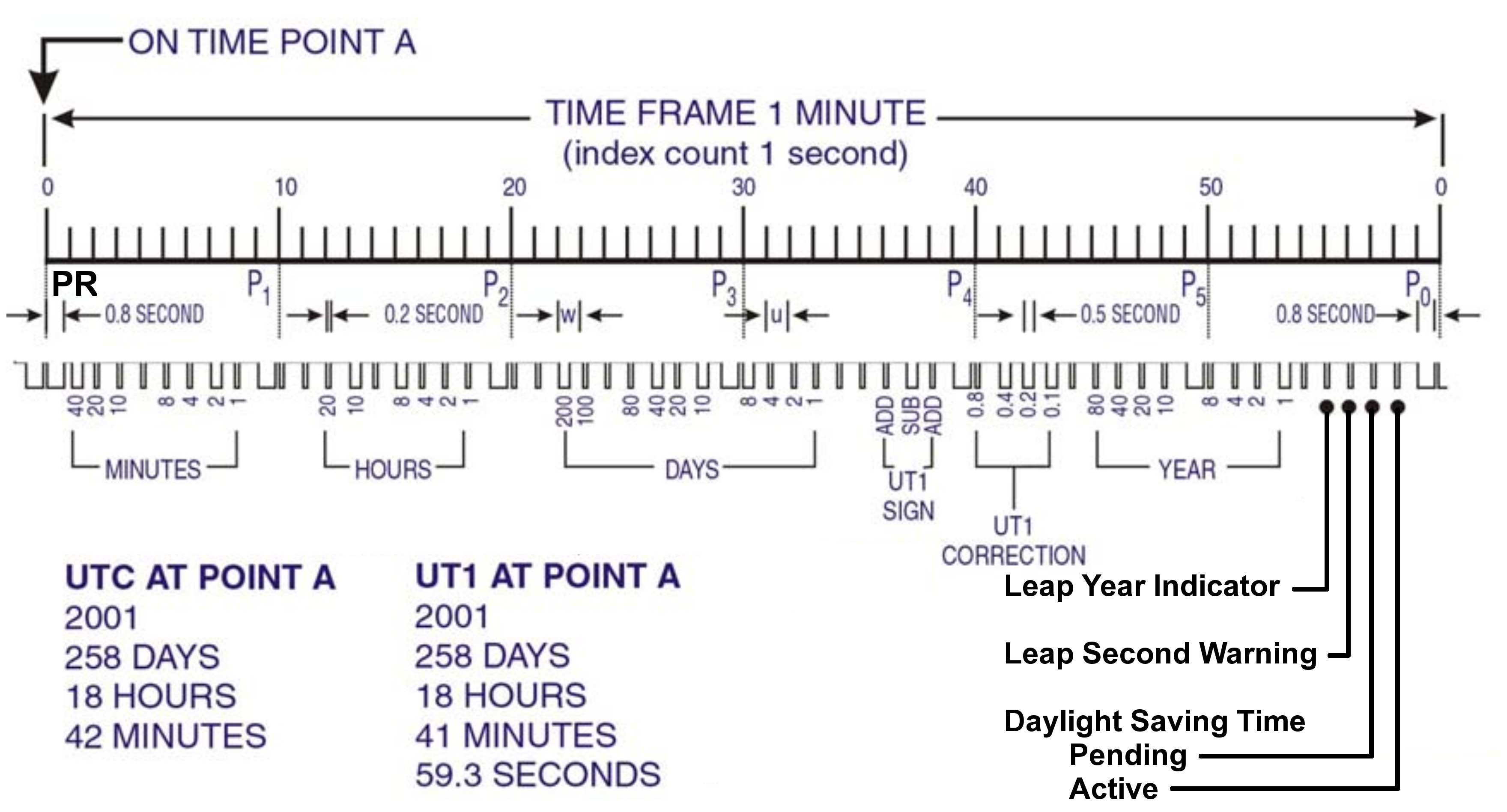
    This is by-and-large the same diagram of the WWVB Time Code Format that you’ll find there, but with:

    • the PR frame reference pulse identified
    • the last four bits clearly labeled
    • some verbiage chopped out
    WWVB Time Code Format - with PR marker
    WWVB Time Code Format – with PR marker

    Memo to Self: Remember that…

    • The time code applies to the minute that’s currently happening, so …
    • The PR pulse happens before the rest of the time code arrives
    • You must know the end-of-month date to apply the leap second bit, but EOM isn’t part of the data stream
  • WWVB Reception Quality: Time From Last Synch

    It occurred to me that a better measure of the WWVB reception quality is the time since the last synch, because that measures the number of consecutive glitch-free minutes, which is a number that’s very difficult to pick out of the Glitchiness vs Time plots.

    A synch occurs only after four consecutive glitch-free frames, with the last three differing only by having properly incrementing minutes based on the first synch. That eliminates successive frames that span hours, as the minutes don’t increment properly from 59 to 00.

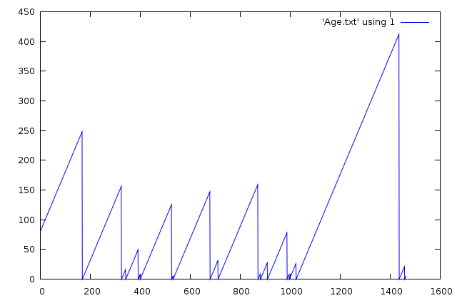
    This is the number of minutes since the most recent synch, versus the number of elapsed minutes, for a 24-hour period starting at UTC 0257 on 25 Dec 2009 (9:57 EST Christmas Eve 2009).

    Synch Age - 24 hrs - 2009-12-24
    Synch Age – 24 hrs – 2009-12-24

    Here’s the spline-smoothed Glitchiness graph I put up yesterday for comparison:

    Glitchiness - splines - 24 hrs - 2009-12-24
    Glitchiness – splines – 24 hrs – 2009-12-24

    An eyeballometric comparison shows my conclusion that synchs happen at the downward spikes in that plot is totally bogus.

    Memo to Self: If you haven’t graphed it, it’s not science yet.

    Useful Bash command:

    grep Age WWVB_2009-12-24a.log | cut -d '=' -f 3 > Age.txt
  • WWVB Reception Quality

    Here on the East Coast of the US, WWVB reception is iffy during the day, due to low signal strength and high ambient noise. Actual data seems hard to come by, so here’s a small contribution.

    This is a plot of the number of glitches per minute, where a glitch is any pulse that’s not within ±60 ms of the expected pulse durations (200, 500, and 800 ms), for a 24-hour period starting at UTC 0257 on 25 Dec 2009 (9:57 EST Christmas Eve 2009). There are 1448 data points, each representing the glitches during the previous minute; each minute starts within 2 seconds of the WWVB on-time frame marker.

    Here’s the raw data, log-scaled on the Y axis to cover the dynamic range. Log scaling can’t handle 0-valued points, so I forced counts of 0 to 0.1 to make them visible.

    Glitchiness - raw - 24 hrs - 2009-12-24
    Glitchiness – raw – 24 hrs – 2009-12-24

    Here’s the same data, Bezier smoothed to make the trends more obvious;  all the points below 1.0 are approximations of a trend toward counts of 0.

    Glitchiness - smoothed - 24 hrs - 2009-12-24
    Glitchiness – smoothed – 24 hrs – 2009-12-24

    Even better, splines show the glitch-free minutes without forcing the data points.

    Glitchiness - splines - 24 hrs - 2009-12-24
    Glitchiness – splines – 24 hrs – 2009-12-24

    My firmware requires four successive glitch-free minutes of reception (plus some additional verification) before synching its local time to WWVB, so it’s exceedingly fussy. Despite that, it still synched 17 times during those 24 hours. The longest free-running time between synchs was 6.8 hours.

    Note that there are 17 downward peaks below 1.0 in that last graph.

    Winter is, of course, the time of best ground-wave propagation from WWVB, so this is about as good as it’s ever going to get.

    Memo to Self: useful Bash and Gnuplot commands…

    
    grep Glitch WWVB_2009-12-24a.log | cut -d H -f 1 > Glitches.txt
    
    set logscale y
    
    set samples 250
    
    plot 'Glitches.txt' using ($2<1?0.1:$2) with points lt 3 pt 2
    
    plot 'Glitches.txt' using 2 smooth csplines with linespoints lt 3 pt 0
    
    
    log-scaled on the Y axis to cover the dynamic range. Log scaling can’t handle 0-valued points, so I forced them to 0.1;
  • Micropositioner Rehabilitation: Z-axis Slide

    With the planetary reducer off, I could remove all the bits and pieces holding the Z-axis slide to the rest of the positioner.

    Rack drive casing
    Rack drive casing

    Note carefully the three spacing washers near each mounting screw. They hold the slide off the casting body by a very precise amount: they’re each 4 mils thick and prone to vanish in a light breeze. I discovered that each screw had three washers when I flicked one off the workbench and discovered two on the floor.

    The metal plate holding the pinion in place has two flat-head screws to the left and two ramps to the right. The conical points of the two long setscrews on the right bear on the ramps, providing a convenient, if obscure from the outside, way to adjust the slide friction by clamping the pinion shaft. One of the setscrews was partially removed, so a previous owner had evidently tried to reduce the overwhelming stickiness.

    With the washers in a safe place, the pinion cover comes off with only slight encouragement.

    Pinion parts
    Pinion parts

    Plenty of congealed lubricating oil to be found.

    Even without the pinion gear, it was exceedingly difficult to urge the two parts of the slide apart: more congealed oil. Much to my surprise, the slide does not have adjustable gibs: it’s one of those precision-ground gadgets that Just Works. This picture shows all the parts in their gunky glory. Note the random dirt in the rack teeth, along with the goo on the pinion shaft.

    Rack and pinion - disassembled
    Rack and pinion – disassembled

    With everything apart, removing the gunk was a simple matter of toxic solvents and mechanical poking with wood picks and splints

    I filed off the burrs on the shafts, thought briefly about grinding some flats for the setscrews, and decided to leave well enough alone.

    A few dabs of clock oil here & there, reassemble everything in reverse order, and the Z-axis moves gracefully with minimal knob torque. It’s very sensitive to the clamping force of those pointed setscrews, though.

    It’s now easy to discover that the planetary reducer has a 5:1 ratio and the Z-axis moves about 6 mm per turn. Because the reducer uses balls, it slips when the slide jams against something, rather than strip its gears.

    I should clean the other two slides, but a dot of clock oil on each cheered them up enough to let me punt that for a while…

    I like it!

    Micropositioner
    Micropositioner
  • Micropositioner Rehabilitation: Planetary Reducer

    Micropositioner
    Micropositioner

    An old 3-axis micropositioner recently found itself on my electronics workbench, where it should come in handy for SMD soldering, microscopic examination, and similar projects requiring the ability to move something in tiny, precise increments. This picture gives you the general idea; it’s mounted on a magnetic base stuck to a random chunk of sheet steel.

    The knob on the front drives the vertical (Z) axis, with the other two controlling the front-to-back (Y) and left-to-right (X) axes. A rotary joint between the X and Y axes, plus another at the tip of the arm, mean you’re not restricted to orthogonal axes; that may be either a blessing or a curse, depending on what you’re trying to accomplish.

    Unfortunately, the Z axis was essentially immovable: that big knurled knob took a remarkable amount of force to drive the slide. Some Quality Shop Time was in order.

    Planetary reducer - cover
    Planetary reducer – cover

    The thing is a chunk of old-school German engineering: nary a gratuitous plastic part to be seen. The planetary reducer has a cast metal cover secured to the torque arm with an acorn nut, which had obviously been removed several times before, as the cover was somewhat chewed beneath the nut.

    I loosened the two setscrews holding the knob in place, gave it a pull, and … nothing. After a protracted struggle and considerable sub-vocal muttering, the knob came off to reveal a thoroughly scarred shaft. Contrary to what I expected, the shaft did not have flats below the setscrews, so the inevitable screw burrs locked the shaft to the knob.

    Planetary reducer - torque arm
    Planetary reducer – torque arm

    The picture to the left shows the planetary drive and torque arm after I filed off the burrs. Two plastic washers (the top one sits on the spring; it’s not shown here) provide smooth bearing surfaces that hold the knob under firm spring pressure, which prevents the Z axis from descending unless you turn the knob manually.

    Planetary drive output shaft screws
    Planetary drive output shaft screws

    Two more setscrews secure the planetary drive’s output bushing to the Z axis pinion shaft. The picture to the right shows that they’re pretty much inaccessible; one was directly behind a tab holding the drive together, the other was aimed at the shoulder of the casting holding the Z axis slide.

    And, of course, even with the knob in place, I can’t turn the mumble shaft, which is why I’m doing this in the first place. The planetary drive uses balls, rather than gears, and the lubricating oil had long since turned into gummy varnish. I slobbered enough light oil into the drive to loosen the gunk enough to make the drive turn-able, albeit with considerable effort. I urged the input shaft barely enough this-a-way and that-a-way to get access to both of the screws.

    Pinion shaft
    Pinion shaft

    As you’d expect, removing the drive required even more muttering and the application of dangerous tools. The pinion shaft was badly scarred in several places, so this poor thing has been dismantled several times before.

    That was entirely enough for one day. Tomorrow, disassembling the Z-axis slide and cleaning things up…