-
Garden Fork Repair
Mary intercepted a complete, albeit defunct, garden fork on its way to the trash and brought it home for repair. It turns out that the handle’s socket had loosened and split around the tine shank, but all the pieces were pretty much in place.
Looks like a job for JB Weld Epoxy!
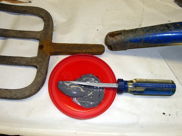
Mix the epoxy with my dedicated mixing screwdriver, butter up the shank, blob the excess epoxy into the socket, shove the parts together, clean off the outside globs, and let it cure overnight.
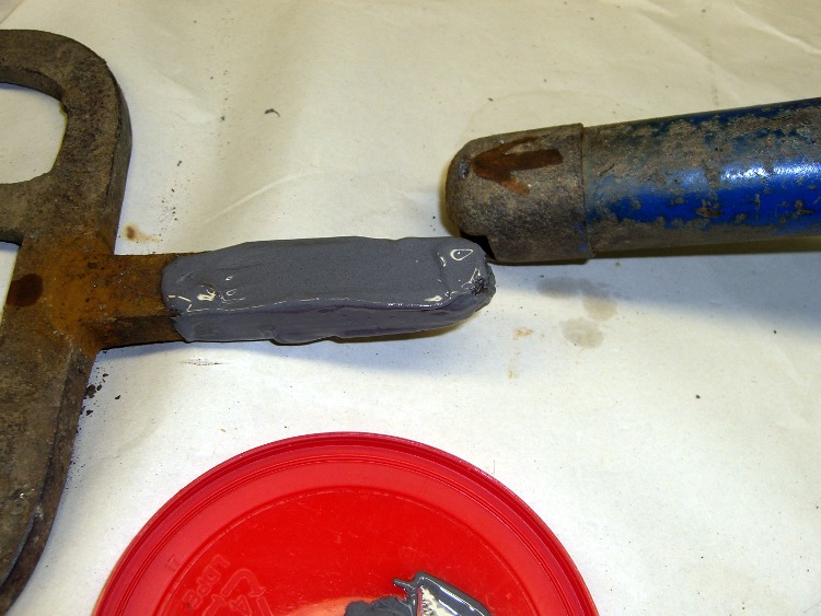
The trick is to get enough epoxy in the socket to fill the voids and mechanically lock the shank in place. This probably won’t work for forks used by burly guys who heave rocks over the horizon, but for our simple needs it’ll do just fine.

Pitchfork repair – epoxy mix 
Pitchfork repair – buttering up the shank Every now and again it’s OK to do an easy repair without a trace of CNC…
-
Subscribe
Subscribed
Already have a WordPress.com account? Log in now.
